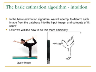
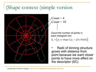
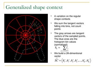
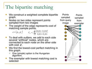
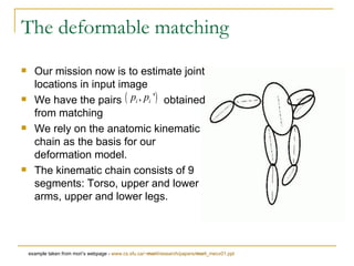
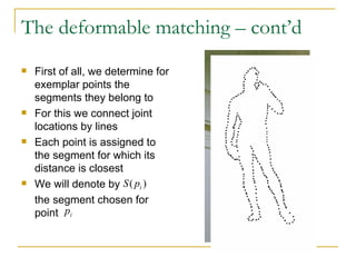
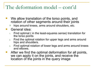
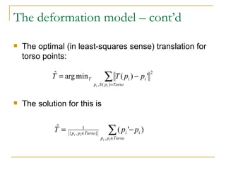
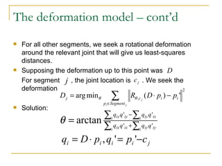
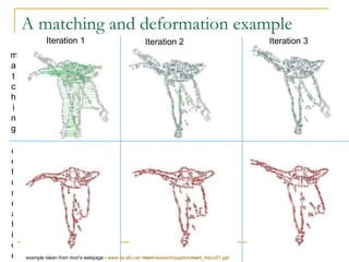
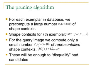
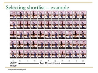
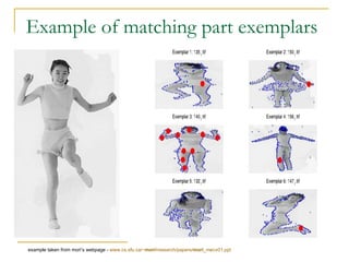
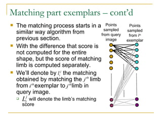
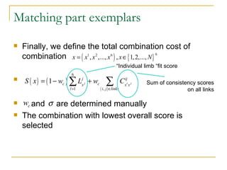
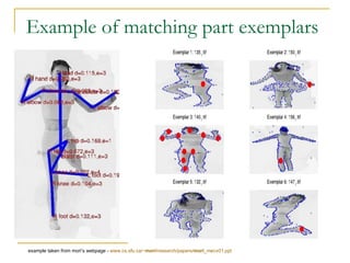
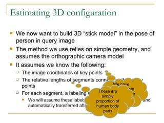
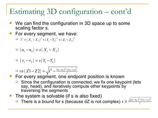
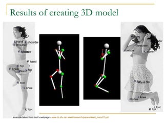
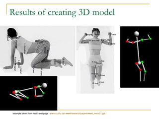
Recovering 3D human body configurations using shape contexts Greg Mori & Jitendra Malik Presented by Joseph Vainshtein Winter 2007
Agenda Motivation and goals The Framework The Basic pose estimation method Pose estimation Estimate joint locations (deformation) Scaling to large image databases Using part examplars 3D Model estimation Some Results
Motivation We receive an image of a person as input What is the person in the image doing?
Motivation – continued We know that there is a person in the input image. We want to recover his body posture to understand the image (what the person in the image is doing) If we had a database of many people in various poses, we could compare our image to the other images. But – It’s not so simple…
Goals Given an input image of a person: Estimate body posture (joint locations) Build 3D model examples taken from Mori’s webpage -  www.cs.sfu.ca/~ mori /research/papers/ mori _mecv01.ppt
Agenda Motivation and goals The Framework The Basic pose estimation method Pose estimation Estimate joint locations (deformation) Scaling to large image databases Using part examplars 3D Model estimation Some Results
The Framework We assume that we have a database of images of people in various poses, photographed from different angles.  In each image in the database, 14 joint locations are manually marked (wrists, elbows, shoulders, hips, knees, ankles, head, waist)
Agenda Motivation and goals The Framework The Basic pose estimation method Pose estimation Estimate joint locations (deformation) Scaling to large image databases Using part examplars 3D Model estimation Some Results
The basic estimation algorithm - intuition In the basic estimation algorithm, we will attempt to deform each image from the database into the input image, and compute a “fit score” Later we will see how to do this more efficiently Query image Database image
The basic estimation algorithm We want to test our input image against some image from our database and obtain a “fit score” Edge detection is applied on each of two images Points are sampled from resulting boundary (300-1000) From now on, we will only work with these points
The basic estimation algorithm The deformation process consist of: Finding a correspondence between points sampled from both images (for every point sampled from boundary of exemplar image find the “best” point on the boundary of input image) Find a deformation of exemplar points into input image This will repeat for several iterations
The shape context A term we will use: shape contexts Shape contexts are point descriptors. They describe the shape around it. In the algorithm we will use a variation: generalized shape contexts. First we will see the simpler variant.
Shape context (simple version) Radii of binning structure grows with distance from point because we want closer points to have more effect on the descriptor (SC) Count = 4 Count = 10 Count the number of points in each histogram bin: example taken from Mori’s webpage -  www.cs.sfu.ca/~ mori /research/papers/ mori _mecv01.ppt
Generalized shape context A variation on the regular shape contexts We sum the tangent vectors falling into bins, not count points The gray arrows are tangent vectors of the sampled points. The blue ones are the histogram bin values (normalized) We build a 2K-dimentional vector
The matching We want to find for every point on the exemplar image it’s corresponding point from the query image.  For each point in exemplar and query image, generalized shape context is calculated. Points with similar descriptors should be matched. The bipartite matching is used for this.
The bipartite matching We construct a weighted complete bipartite graph. Nodes on two sides represent points sampled from two images  The weight of the edge represents cost of matching sample points.  To deal with outliers, we add to each side several “artificial” nodes, which are connected to each node on the other side with cost  . We find the lowest-cost perfect matching in this graph. One (simple) option is the Hungarian algorithm.  The exemplar with lowest matching cost is selected Points sampled from exemplar Points sampled from query image
Our mission now is to estimate joint locations in input image We have the pairs  obtained from matching We rely on the anatomic kinematic chain as the basis for our deformation model. The kinematic chain consists of 9 segments: Torso, upper and lower arms, upper and lower legs. The deformable matching example taken from mori’s webpage -  www.cs.sfu.ca/~ mori /research/papers/ mori _mecv01.ppt
The deformable matching – cont’d First of all, we determine for exemplar points the segments they belong to For this we connect joint locations by lines Each point is assigned to the segment for which its distance is closest We will denote by  the segment chosen for point
The deformation model – cont’d We allow translation of the torso points, and rotation of other segments around their joints  hips around knees, arms around shoulders, etc. General idea: Find optimal ( in the least-squares sense) translation for the torso points Find the optimal rotation for upper legs and arms around hips and shoulders. Find optimal rotation of lower legs and arms around knees and elbows. After we find the optimal deformation for all points, we can apply it on the joints, and receive the location of the joints in the query image
The optimal (in least-squares sense) translation for torso points: The solution for this is The deformation model – cont’d
The deformation model – cont’d For all other segments, we seek a rotational deformation around the relevant joint that will give us least-squares distances. Supposing the deformation up to this point was  For segment  , the joint location is  . We seek the deformation Solution:
The deformation model – cont’d The process is repeated for a small number of iterations (point matching and deformation)  Joint locations in input image are found by applying optimal deformation on joints from exemplar We also have a score for the fit we have made: matching cost for the optimal assignment
A matching and deformation example Query image points Exemplar points example taken from mori’s webpage -  www.cs.sfu.ca/~ mori /research/papers/ mori _mecv01.ppt
A matching and deformation example Iteration 1 Iteration 3 Iteration 2 matching deformation example taken from mori’s webpage -  www.cs.sfu.ca/~ mori /research/papers/ mori _mecv01.ppt
Agenda Motivation and goals The Framework The Basic pose estimation method Pose estimation Estimate joint locations (deformation) Scaling to large image databases Using part examplars 3D Model estimation Some Results
Scaling to large exemplar databases The simplest algorithm one can think of: Run basic algorithm on all images in database, for each one obtain matching score Choose image with best score This is not applicable in systems with large exemplar databases, which are needed if we want to not to restrict the algorithm to specific body postures We will present a method to solve this.
Scaling to large exemplar databases The idea : If the query image and the exemplar image are very different, there is no need to run the smart and expensive algorithm to find that this is a bad fit.  Solution: Use a pruning algorithm to obtain a short list of “good” candidate images, then perform expensive and more accurate algorithm on each.
The pruning algorithm For each exemplar in database, we precompute a large number  of   shape contexts Shape contexts for  i ’th exemplar: For the query image we compute only a small number  of  representative  shape contexts, These will be enough to “disqualify” bad candidates
The pruning algorithm – cont’d For those  representatives, we find the best  matches from the precomputed shape contexts. For representative  best match from i’th exemplar is  : The distance between shape context vectors is computed using the same formula as in matching cost:
The pruning algorithm – cont’d Now we estimate distance between the shapes as normalized sum of matching cost of the r representative points is a normalizing factor If representative number u was not a good representative point, we want it to have less effect on the cost
The pruning algorithm – cont’d The shortlist of candidates is selected by sorting the exemplars by distance from query image The basic algorithm is performed on the shortlist to find the best match
Selecting shortlist – example Query image Top 10 candidates example taken from the paper
Agenda Motivation and goals The Framework The Basic pose estimation method Pose estimation Estimate joint locations (deformation) Scaling to large image databases Using part examplars 3D Model estimation Some Results
Matching part exemplars - motivation When using the algorithm presented above in a general matching framework (not restricted to specific body positions and camera angles) a very large image database is needed to succeed. In this section we will show a method to reduce the exemplar database needed to match the shape. This will also reduce runtime
Matching part exemplars - intuition The idea here is not to match the entire shape, but to match the different body parts independently The resulting match might include body parts matched from different images We allow six “limbs” as body parts: Left and right arms Left and right legs Waist Head
Example of matching part exemplars  example taken from mori’s webpage -  www.cs.sfu.ca/~ mori /research/papers/ mori _mecv01.ppt
Matching part exemplars – cont’d The matching process starts in a similar way algorithm from previous section. With the difference that score is not computed for the entire shape, but the score of matching limb is computed separately. We’ll denote by  the matching obtained by matching the  limb from  exemplar to  limb in query image. will denote the limb’s matching score  Points sampled from i th  exemplar Points sampled from query image
Matching part exemplars – cont’d We now want to find a combination of these separate limbs into a match for the entire shape. The first idea that comes to mind is simply to choose for each limb the exemplar with highest score This is not a good idea, since in this simple manner nothing enforces the combination to be consistent Solution: Define a measure of consistency for a combination Then, create a score that will take into account both the consistency score and the individual matching score for limbs
Matching part exemplars:  consistency score A combination is consistent if limbs are at “proper” distances from one another  Our measure of consistency will use the distances between limb base points shoulders for arms, hips for legs, for waist and head they are just the points We will enforce the following distances to be “proper”: Left arm – head Right arm – head Waist-head Left leg – waist Right leg - waist
Matching part exemplars:  consistency score – cont’d A combination of two limbs is consistent if the distance between them in the combination is comparable to the distance between those limbs in the original images The consistency score of some combination will be sum of consistency scores across links For each of the links, we try all  matching options, and compute the distance between bases in every matching option. This could even be computed in advance.
Matching part exemplars: consistency score – cont’d We define  as the consistency cost of combining limb  from exemplar  and limb  from exemplar  is the 2D distance between limb bases is a link Note that as distance  deviates from consistent exemplars,  increases exponentially
Matching part exemplars Finally, we define the total combination cost of combination and  are determined manually The combination with lowest overall score is selected Individual limb “fit score” Sum of consistency scores on all links
Example of matching part exemplars  example taken from mori’s webpage -  www.cs.sfu.ca/~ mori /research/papers/ mori _mecv01.ppt
Agenda Motivation and goals The Model The Basic pose estimation method Point sampling The shape context & generalized shape context The point matching  Shape deformation Scaling the algorithm to large image databases Matching part examplars 3D Model estimation Some Results
Estimating 3D configuration We now want to build 3D “stick model” in the pose of person in query image The method we use relies on simple geometry, and assumes the orthographic camera model It assumes we know the following: The image coordinates of key points The relative lengths of segments connecting these key points For each segment, a labeling of “closer endpoint” We will assume these labels are supplied on exemplars, and automatically transferred after the matching process We have obtained them in the algorithm from previous sections These are simply proportion of human body parts
Estimating 3D configuration – cont’d We can find the configuration in 3D space up to some scaling factor s. For every segment, we have: For every segment, one endpoint position is known Since the configuration is connected, we fix one keypoint (lets say, head), and iteratively compute other keypoints by traversing the segments The system is solvable (if s is also fixed) There is a bound for s (because dZ is not complex)
Agenda Motivation and goals The Model The Basic pose estimation method Point sampling The shape context & generalized shape context The point matching  Shape deformation Scaling the algorithm to large image databases Matching part examplars 3D Model estimation Some Results
Results of creating 3D model example taken from mori’s webpage -  www.cs.sfu.ca/~ mori /research/papers/ mori _mecv01.ppt
Questions Now’s the time for your questions… ? example taken from mori’s webpage -  www.cs.sfu.ca/~ mori /research/papers/ mori _mecv01.ppt
Bibliography & credits  Some results and a few slides were taken from Mori’s webpage www.cs.sfu.ca/~ mori /research/papers/ mori _mecv01.ppt A slightly different version of the paper can also be found there http://www.cs.sfu.ca/~mori/courses/cmpt882/papers/mori-eccv02.pdf

Recovering 3D human body configurations using shape contexts

  • 1.
    Recovering 3D humanbody configurations using shape contexts Greg Mori & Jitendra Malik Presented by Joseph Vainshtein Winter 2007
  • 2.
    Agenda Motivation andgoals The Framework The Basic pose estimation method Pose estimation Estimate joint locations (deformation) Scaling to large image databases Using part examplars 3D Model estimation Some Results
  • 3.
    Motivation We receivean image of a person as input What is the person in the image doing?
  • 4.
    Motivation – continuedWe know that there is a person in the input image. We want to recover his body posture to understand the image (what the person in the image is doing) If we had a database of many people in various poses, we could compare our image to the other images. But – It’s not so simple…
  • 5.
    Goals Given aninput image of a person: Estimate body posture (joint locations) Build 3D model examples taken from Mori’s webpage - www.cs.sfu.ca/~ mori /research/papers/ mori _mecv01.ppt
  • 6.
    Agenda Motivation andgoals The Framework The Basic pose estimation method Pose estimation Estimate joint locations (deformation) Scaling to large image databases Using part examplars 3D Model estimation Some Results
  • 7.
    The Framework Weassume that we have a database of images of people in various poses, photographed from different angles. In each image in the database, 14 joint locations are manually marked (wrists, elbows, shoulders, hips, knees, ankles, head, waist)
  • 8.
    Agenda Motivation andgoals The Framework The Basic pose estimation method Pose estimation Estimate joint locations (deformation) Scaling to large image databases Using part examplars 3D Model estimation Some Results
  • 9.
    The basic estimationalgorithm - intuition In the basic estimation algorithm, we will attempt to deform each image from the database into the input image, and compute a “fit score” Later we will see how to do this more efficiently Query image Database image
  • 10.
    The basic estimationalgorithm We want to test our input image against some image from our database and obtain a “fit score” Edge detection is applied on each of two images Points are sampled from resulting boundary (300-1000) From now on, we will only work with these points
  • 11.
    The basic estimationalgorithm The deformation process consist of: Finding a correspondence between points sampled from both images (for every point sampled from boundary of exemplar image find the “best” point on the boundary of input image) Find a deformation of exemplar points into input image This will repeat for several iterations
  • 12.
    The shape contextA term we will use: shape contexts Shape contexts are point descriptors. They describe the shape around it. In the algorithm we will use a variation: generalized shape contexts. First we will see the simpler variant.
  • 13.
    Shape context (simpleversion) Radii of binning structure grows with distance from point because we want closer points to have more effect on the descriptor (SC) Count = 4 Count = 10 Count the number of points in each histogram bin: example taken from Mori’s webpage - www.cs.sfu.ca/~ mori /research/papers/ mori _mecv01.ppt
  • 14.
    Generalized shape contextA variation on the regular shape contexts We sum the tangent vectors falling into bins, not count points The gray arrows are tangent vectors of the sampled points. The blue ones are the histogram bin values (normalized) We build a 2K-dimentional vector
  • 15.
    The matching Wewant to find for every point on the exemplar image it’s corresponding point from the query image. For each point in exemplar and query image, generalized shape context is calculated. Points with similar descriptors should be matched. The bipartite matching is used for this.
  • 16.
    The bipartite matchingWe construct a weighted complete bipartite graph. Nodes on two sides represent points sampled from two images The weight of the edge represents cost of matching sample points. To deal with outliers, we add to each side several “artificial” nodes, which are connected to each node on the other side with cost . We find the lowest-cost perfect matching in this graph. One (simple) option is the Hungarian algorithm. The exemplar with lowest matching cost is selected Points sampled from exemplar Points sampled from query image
  • 17.
    Our mission nowis to estimate joint locations in input image We have the pairs obtained from matching We rely on the anatomic kinematic chain as the basis for our deformation model. The kinematic chain consists of 9 segments: Torso, upper and lower arms, upper and lower legs. The deformable matching example taken from mori’s webpage - www.cs.sfu.ca/~ mori /research/papers/ mori _mecv01.ppt
  • 18.
    The deformable matching– cont’d First of all, we determine for exemplar points the segments they belong to For this we connect joint locations by lines Each point is assigned to the segment for which its distance is closest We will denote by the segment chosen for point
  • 19.
    The deformation model– cont’d We allow translation of the torso points, and rotation of other segments around their joints hips around knees, arms around shoulders, etc. General idea: Find optimal ( in the least-squares sense) translation for the torso points Find the optimal rotation for upper legs and arms around hips and shoulders. Find optimal rotation of lower legs and arms around knees and elbows. After we find the optimal deformation for all points, we can apply it on the joints, and receive the location of the joints in the query image
  • 20.
    The optimal (inleast-squares sense) translation for torso points: The solution for this is The deformation model – cont’d
  • 21.
    The deformation model– cont’d For all other segments, we seek a rotational deformation around the relevant joint that will give us least-squares distances. Supposing the deformation up to this point was For segment , the joint location is . We seek the deformation Solution:
  • 22.
    The deformation model– cont’d The process is repeated for a small number of iterations (point matching and deformation) Joint locations in input image are found by applying optimal deformation on joints from exemplar We also have a score for the fit we have made: matching cost for the optimal assignment
  • 23.
    A matching anddeformation example Query image points Exemplar points example taken from mori’s webpage - www.cs.sfu.ca/~ mori /research/papers/ mori _mecv01.ppt
  • 24.
    A matching anddeformation example Iteration 1 Iteration 3 Iteration 2 matching deformation example taken from mori’s webpage - www.cs.sfu.ca/~ mori /research/papers/ mori _mecv01.ppt
  • 25.
    Agenda Motivation andgoals The Framework The Basic pose estimation method Pose estimation Estimate joint locations (deformation) Scaling to large image databases Using part examplars 3D Model estimation Some Results
  • 26.
    Scaling to largeexemplar databases The simplest algorithm one can think of: Run basic algorithm on all images in database, for each one obtain matching score Choose image with best score This is not applicable in systems with large exemplar databases, which are needed if we want to not to restrict the algorithm to specific body postures We will present a method to solve this.
  • 27.
    Scaling to largeexemplar databases The idea : If the query image and the exemplar image are very different, there is no need to run the smart and expensive algorithm to find that this is a bad fit. Solution: Use a pruning algorithm to obtain a short list of “good” candidate images, then perform expensive and more accurate algorithm on each.
  • 28.
    The pruning algorithmFor each exemplar in database, we precompute a large number of shape contexts Shape contexts for i ’th exemplar: For the query image we compute only a small number of representative shape contexts, These will be enough to “disqualify” bad candidates
  • 29.
    The pruning algorithm– cont’d For those representatives, we find the best matches from the precomputed shape contexts. For representative best match from i’th exemplar is : The distance between shape context vectors is computed using the same formula as in matching cost:
  • 30.
    The pruning algorithm– cont’d Now we estimate distance between the shapes as normalized sum of matching cost of the r representative points is a normalizing factor If representative number u was not a good representative point, we want it to have less effect on the cost
  • 31.
    The pruning algorithm– cont’d The shortlist of candidates is selected by sorting the exemplars by distance from query image The basic algorithm is performed on the shortlist to find the best match
  • 32.
    Selecting shortlist –example Query image Top 10 candidates example taken from the paper
  • 33.
    Agenda Motivation andgoals The Framework The Basic pose estimation method Pose estimation Estimate joint locations (deformation) Scaling to large image databases Using part examplars 3D Model estimation Some Results
  • 34.
    Matching part exemplars- motivation When using the algorithm presented above in a general matching framework (not restricted to specific body positions and camera angles) a very large image database is needed to succeed. In this section we will show a method to reduce the exemplar database needed to match the shape. This will also reduce runtime
  • 35.
    Matching part exemplars- intuition The idea here is not to match the entire shape, but to match the different body parts independently The resulting match might include body parts matched from different images We allow six “limbs” as body parts: Left and right arms Left and right legs Waist Head
  • 36.
    Example of matchingpart exemplars example taken from mori’s webpage - www.cs.sfu.ca/~ mori /research/papers/ mori _mecv01.ppt
  • 37.
    Matching part exemplars– cont’d The matching process starts in a similar way algorithm from previous section. With the difference that score is not computed for the entire shape, but the score of matching limb is computed separately. We’ll denote by the matching obtained by matching the limb from exemplar to limb in query image. will denote the limb’s matching score Points sampled from i th exemplar Points sampled from query image
  • 38.
    Matching part exemplars– cont’d We now want to find a combination of these separate limbs into a match for the entire shape. The first idea that comes to mind is simply to choose for each limb the exemplar with highest score This is not a good idea, since in this simple manner nothing enforces the combination to be consistent Solution: Define a measure of consistency for a combination Then, create a score that will take into account both the consistency score and the individual matching score for limbs
  • 39.
    Matching part exemplars: consistency score A combination is consistent if limbs are at “proper” distances from one another Our measure of consistency will use the distances between limb base points shoulders for arms, hips for legs, for waist and head they are just the points We will enforce the following distances to be “proper”: Left arm – head Right arm – head Waist-head Left leg – waist Right leg - waist
  • 40.
    Matching part exemplars: consistency score – cont’d A combination of two limbs is consistent if the distance between them in the combination is comparable to the distance between those limbs in the original images The consistency score of some combination will be sum of consistency scores across links For each of the links, we try all matching options, and compute the distance between bases in every matching option. This could even be computed in advance.
  • 41.
    Matching part exemplars:consistency score – cont’d We define as the consistency cost of combining limb from exemplar and limb from exemplar is the 2D distance between limb bases is a link Note that as distance deviates from consistent exemplars, increases exponentially
  • 42.
    Matching part exemplarsFinally, we define the total combination cost of combination and are determined manually The combination with lowest overall score is selected Individual limb “fit score” Sum of consistency scores on all links
  • 43.
    Example of matchingpart exemplars example taken from mori’s webpage - www.cs.sfu.ca/~ mori /research/papers/ mori _mecv01.ppt
  • 44.
    Agenda Motivation andgoals The Model The Basic pose estimation method Point sampling The shape context & generalized shape context The point matching Shape deformation Scaling the algorithm to large image databases Matching part examplars 3D Model estimation Some Results
  • 45.
    Estimating 3D configurationWe now want to build 3D “stick model” in the pose of person in query image The method we use relies on simple geometry, and assumes the orthographic camera model It assumes we know the following: The image coordinates of key points The relative lengths of segments connecting these key points For each segment, a labeling of “closer endpoint” We will assume these labels are supplied on exemplars, and automatically transferred after the matching process We have obtained them in the algorithm from previous sections These are simply proportion of human body parts
  • 46.
    Estimating 3D configuration– cont’d We can find the configuration in 3D space up to some scaling factor s. For every segment, we have: For every segment, one endpoint position is known Since the configuration is connected, we fix one keypoint (lets say, head), and iteratively compute other keypoints by traversing the segments The system is solvable (if s is also fixed) There is a bound for s (because dZ is not complex)
  • 47.
    Agenda Motivation andgoals The Model The Basic pose estimation method Point sampling The shape context & generalized shape context The point matching Shape deformation Scaling the algorithm to large image databases Matching part examplars 3D Model estimation Some Results
  • 48.
    Results of creating3D model example taken from mori’s webpage - www.cs.sfu.ca/~ mori /research/papers/ mori _mecv01.ppt
  • 49.
    Results of creating3D model example taken from mori’s webpage - www.cs.sfu.ca/~ mori /research/papers/ mori _mecv01.ppt
  • 50.
    Questions Now’s thetime for your questions… ? example taken from mori’s webpage - www.cs.sfu.ca/~ mori /research/papers/ mori _mecv01.ppt
  • 51.
    Bibliography & credits Some results and a few slides were taken from Mori’s webpage www.cs.sfu.ca/~ mori /research/papers/ mori _mecv01.ppt A slightly different version of the paper can also be found there http://www.cs.sfu.ca/~mori/courses/cmpt882/papers/mori-eccv02.pdf