Download as PDF, PPTX
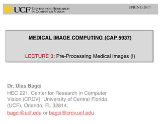
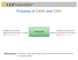
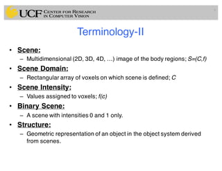
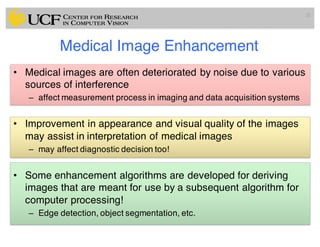
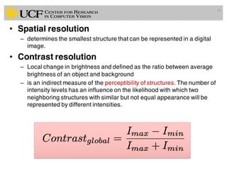
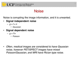
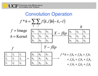
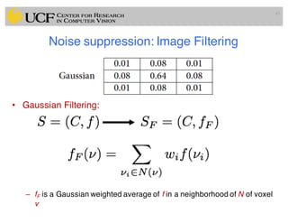
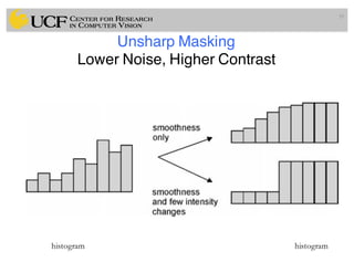
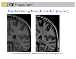
![Median Filtering (Details)
48
[8 8 8 8 8 8 8 8 255]
median](https://image.slidesharecdn.com/lec3-170330052248/85/Lec3-Pre-Processing-Medical-Images-48-320.jpg)
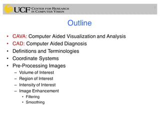
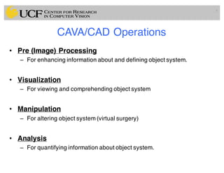
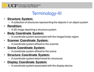
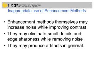
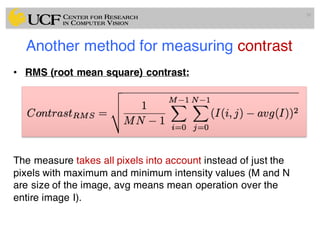
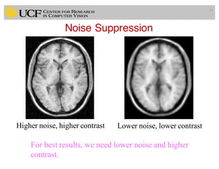
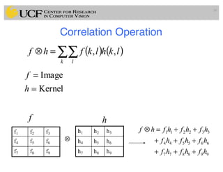
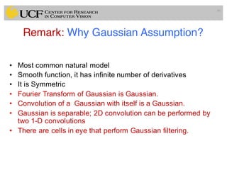
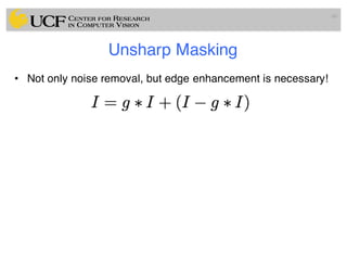
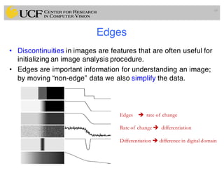
![Filtering Operation (Spatial Domain)
49
111
111
111
],[g ⋅⋅
Example: Box Filtering
(smoothing)
What does it do?
• Replaces each pixel with an
average of its neighborhood
• Achieve smoothing effect
(remove sharp features)](https://image.slidesharecdn.com/lec3-170330052248/85/Lec3-Pre-Processing-Medical-Images-49-320.jpg)
![0 0 0 0 0 0 0 0 0 0
0 0 0 0 0 0 0 0 0 0
0 0 0 90 90 90 90 90 0 0
0 0 0 90 90 90 90 90 0 0
0 0 0 90 90 90 90 90 0 0
0 0 0 90 0 90 90 90 0 0
0 0 0 90 90 90 90 90 0 0
0 0 0 0 0 0 0 0 0 0
0 0 90 0 0 0 0 0 0 0
0 0 0 0 0 0 0 0 0 0
0
0 0 0 0 0 0 0 0 0 0
0 0 0 0 0 0 0 0 0 0
0 0 0 90 90 90 90 90 0 0
0 0 0 90 90 90 90 90 0 0
0 0 0 90 90 90 90 90 0 0
0 0 0 90 0 90 90 90 0 0
0 0 0 90 90 90 90 90 0 0
0 0 0 0 0 0 0 0 0 0
0 0 90 0 0 0 0 0 0 0
0 0 0 0 0 0 0 0 0 0
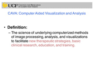
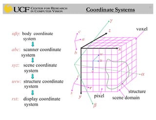
Credit: S. Seitz
],[],[],[
,
lnkmflkgnmh
lk
++= ∑
[.,.]h[.,.]f
111
111
111
],[g ⋅⋅
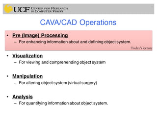
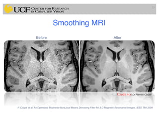
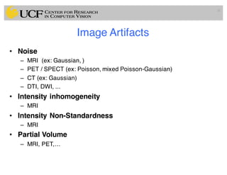
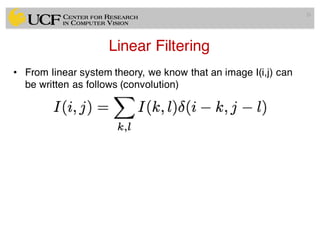
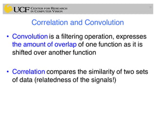
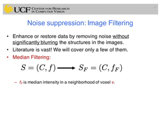
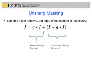
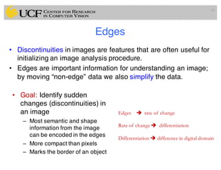
Filtering Operation (Spatial Domain)](https://image.slidesharecdn.com/lec3-170330052248/85/Lec3-Pre-Processing-Medical-Images-50-320.jpg)
![0 0 0 0 0 0 0 0 0 0
0 0 0 0 0 0 0 0 0 0
0 0 0 90 90 90 90 90 0 0
0 0 0 90 90 90 90 90 0 0
0 0 0 90 90 90 90 90 0 0
0 0 0 90 0 90 90 90 0 0
0 0 0 90 90 90 90 90 0 0
0 0 0 0 0 0 0 0 0 0
0 0 90 0 0 0 0 0 0 0
0 0 0 0 0 0 0 0 0 0
0 10
0 0 0 0 0 0 0 0 0 0
0 0 0 0 0 0 0 0 0 0
0 0 0 90 90 90 90 90 0 0
0 0 0 90 90 90 90 90 0 0
0 0 0 90 90 90 90 90 0 0
0 0 0 90 0 90 90 90 0 0
0 0 0 90 90 90 90 90 0 0
0 0 0 0 0 0 0 0 0 0
0 0 90 0 0 0 0 0 0 0
0 0 0 0 0 0 0 0 0 0
[.,.]h[.,.]f
111
111
111
],[g ⋅⋅
Credit: S. Seitz
],[],[],[
,
lnkmflkgnmh
lk
++= ∑
Filtering Operation (Spatial Domain)](https://image.slidesharecdn.com/lec3-170330052248/85/Lec3-Pre-Processing-Medical-Images-51-320.jpg)
![0 0 0 0 0 0 0 0 0 0
0 0 0 0 0 0 0 0 0 0
0 0 0 90 90 90 90 90 0 0
0 0 0 90 90 90 90 90 0 0
0 0 0 90 90 90 90 90 0 0
0 0 0 90 0 90 90 90 0 0
0 0 0 90 90 90 90 90 0 0
0 0 0 0 0 0 0 0 0 0
0 0 90 0 0 0 0 0 0 0
0 0 0 0 0 0 0 0 0 0
0 10 20
0 0 0 0 0 0 0 0 0 0
0 0 0 0 0 0 0 0 0 0
0 0 0 90 90 90 90 90 0 0
0 0 0 90 90 90 90 90 0 0
0 0 0 90 90 90 90 90 0 0
0 0 0 90 0 90 90 90 0 0
0 0 0 90 90 90 90 90 0 0
0 0 0 0 0 0 0 0 0 0
0 0 90 0 0 0 0 0 0 0
0 0 0 0 0 0 0 0 0 0
[.,.]h[.,.]f
111
111
111
],[g ⋅⋅
Credit: S. Seitz
],[],[],[
,
lnkmflkgnmh
lk
++= ∑
Filtering Operation (Spatial Domain)](https://image.slidesharecdn.com/lec3-170330052248/85/Lec3-Pre-Processing-Medical-Images-52-320.jpg)
![0 0 0 0 0 0 0 0 0 0
0 0 0 0 0 0 0 0 0 0
0 0 0 90 90 90 90 90 0 0
0 0 0 90 90 90 90 90 0 0
0 0 0 90 90 90 90 90 0 0
0 0 0 90 0 90 90 90 0 0
0 0 0 90 90 90 90 90 0 0
0 0 0 0 0 0 0 0 0 0
0 0 90 0 0 0 0 0 0 0
0 0 0 0 0 0 0 0 0 0
0 10 20 30
0 0 0 0 0 0 0 0 0 0
0 0 0 0 0 0 0 0 0 0
0 0 0 90 90 90 90 90 0 0
0 0 0 90 90 90 90 90 0 0
0 0 0 90 90 90 90 90 0 0
0 0 0 90 0 90 90 90 0 0
0 0 0 90 90 90 90 90 0 0
0 0 0 0 0 0 0 0 0 0
0 0 90 0 0 0 0 0 0 0
0 0 0 0 0 0 0 0 0 0
[.,.]h[.,.]f
111
111
111
],[g ⋅⋅
Credit: S. Seitz
],[],[],[
,
lnkmflkgnmh
lk
++= ∑
Filtering Operation (Spatial Domain)](https://image.slidesharecdn.com/lec3-170330052248/85/Lec3-Pre-Processing-Medical-Images-53-320.jpg)
![0 10 20 30 30
0 0 0 0 0 0 0 0 0 0
0 0 0 0 0 0 0 0 0 0
0 0 0 90 90 90 90 90 0 0
0 0 0 90 90 90 90 90 0 0
0 0 0 90 90 90 90 90 0 0
0 0 0 90 0 90 90 90 0 0
0 0 0 90 90 90 90 90 0 0
0 0 0 0 0 0 0 0 0 0
0 0 90 0 0 0 0 0 0 0
0 0 0 0 0 0 0 0 0 0
[.,.]h[.,.]f
111
111
111
],[g ⋅⋅
Credit: S. Seitz
],[],[],[
,
lnkmflkgnmh
lk
++= ∑
Filtering Operation (Spatial Domain)](https://image.slidesharecdn.com/lec3-170330052248/85/Lec3-Pre-Processing-Medical-Images-54-320.jpg)
![0 10 20 30 30
0 0 0 0 0 0 0 0 0 0
0 0 0 0 0 0 0 0 0 0
0 0 0 90 90 90 90 90 0 0
0 0 0 90 90 90 90 90 0 0
0 0 0 90 90 90 90 90 0 0
0 0 0 90 0 90 90 90 0 0
0 0 0 90 90 90 90 90 0 0
0 0 0 0 0 0 0 0 0 0
0 0 90 0 0 0 0 0 0 0
0 0 0 0 0 0 0 0 0 0
[.,.]h[.,.]f
111
111
111
],[g ⋅⋅
Credit: S. Seitz
?
],[],[],[
,
lnkmflkgnmh
lk
++= ∑
Filtering Operation (Spatial Domain)](https://image.slidesharecdn.com/lec3-170330052248/85/Lec3-Pre-Processing-Medical-Images-55-320.jpg)
![0 10 20 30 30
50
0 0 0 0 0 0 0 0 0 0
0 0 0 0 0 0 0 0 0 0
0 0 0 90 90 90 90 90 0 0
0 0 0 90 90 90 90 90 0 0
0 0 0 90 90 90 90 90 0 0
0 0 0 90 0 90 90 90 0 0
0 0 0 90 90 90 90 90 0 0
0 0 0 0 0 0 0 0 0 0
0 0 90 0 0 0 0 0 0 0
0 0 0 0 0 0 0 0 0 0
[.,.]h[.,.]f
111
111
111
],[g ⋅⋅
Credit: S. Seitz
?
],[],[],[
,
lnkmflkgnmh
lk
++= ∑
Filtering Operation (Spatial Domain)](https://image.slidesharecdn.com/lec3-170330052248/85/Lec3-Pre-Processing-Medical-Images-56-320.jpg)
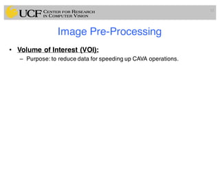
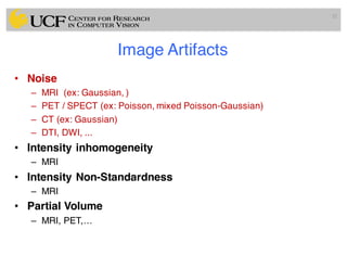
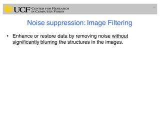
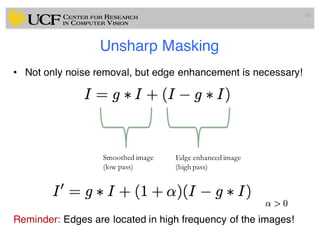
![0 0 0 0 0 0 0 0 0 0
0 0 0 0 0 0 0 0 0 0
0 0 0 90 90 90 90 90 0 0
0 0 0 90 90 90 90 90 0 0
0 0 0 90 90 90 90 90 0 0
0 0 0 90 0 90 90 90 0 0
0 0 0 90 90 90 90 90 0 0
0 0 0 0 0 0 0 0 0 0
0 0 90 0 0 0 0 0 0 0
0 0 0 0 0 0 0 0 0 0
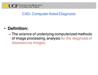
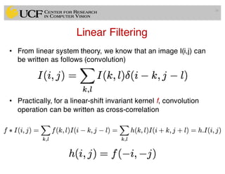
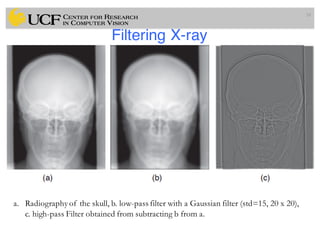
0 10 20 30 30 30 20 10
0 20 40 60 60 60 40 20
0 30 60 90 90 90 60 30
0 30 50 80 80 90 60 30
0 30 50 80 80 90 60 30
0 20 30 50 50 60 40 20
10 20 30 30 30 30 20 10
10 10 10 0 0 0 0 0
[.,.]h[.,.]f
111
111
111
],[g ⋅⋅
Credit: S. Seitz
],[],[],[
,
lnkmflkgnmh
lk
++= ∑
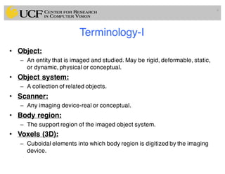
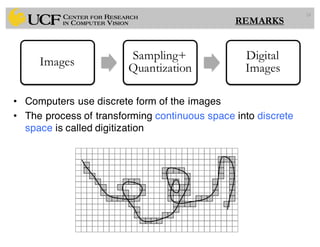
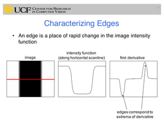
Filtering Operation (Spatial Domain)](https://image.slidesharecdn.com/lec3-170330052248/85/Lec3-Pre-Processing-Medical-Images-57-320.jpg)
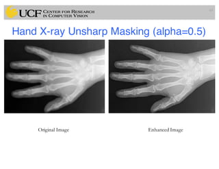
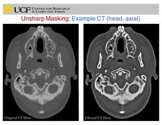
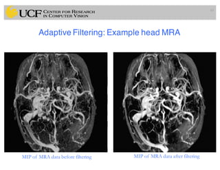
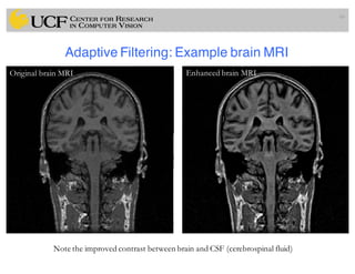
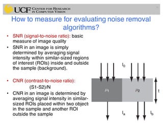
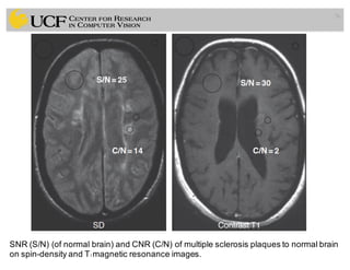
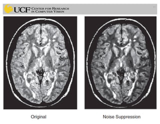
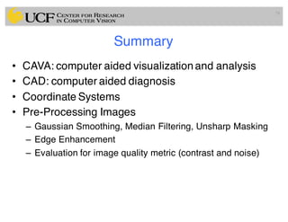

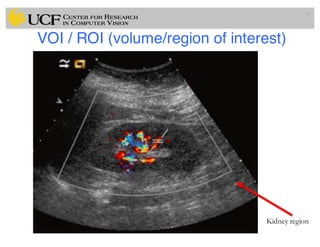
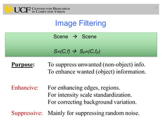
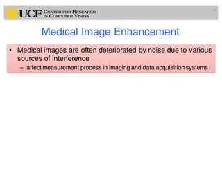
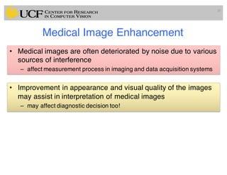
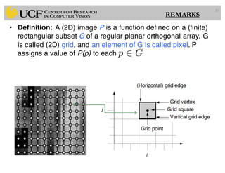
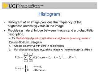
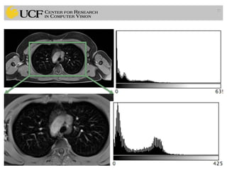
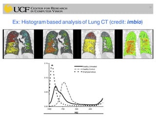
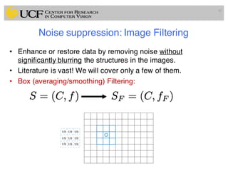
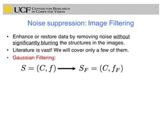
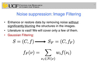
The lecture covers the fundamentals of medical image computing, focusing on pre-processing medical images, including definitions, terminologies, and techniques such as volume of interest, region of interest, and various filtering methods. It discusses the importance of computer-aided visualization and diagnosis in enhancing the quality of medical images for improved analysis and decision-making. Various noise suppression and enhancement techniques, such as Gaussian and median filtering, are also explored to enhance image quality for better diagnostic outcomes.