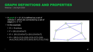
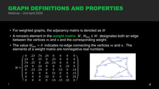
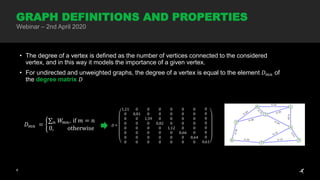
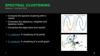
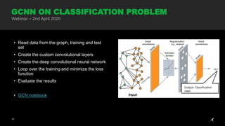
The document discusses graph neural networks, focusing on graph definitions, properties, and applications such as spectral clustering and graph convolutional neural networks. It covers key concepts like adjacency matrices, graph Laplacians, and how they are used in convolutional filters for classification tasks. The webinar on April 2nd, 2020, also includes practical demonstrations of clustering techniques and deep learning models related to graph processing.

1. GRAPH NEURAL
NETWORKS
Luca Crociani (Machine Learning Reply)
Francesco Tangari (Machine Learning Reply)

2. 2
1. Graph definitions and properties
2. Graph spectrum
3. Laplacian convolutional filter
4. Graph Convolutional Neural Networks
1. Spectral clustering in practice
2. Graph Convolution in practice
3. GCNN on classification problem
TODAY’S AGENDA
Webinar – 2nd April 2020
THEORY PRACTICE

3. 3
• A graph 𝐺 = {𝑉, 𝐵} is defined as a set of
vertices 𝑉, which are connected by a set of
edges 𝐵 ⊂ 𝑉 × 𝑉
• In this example:
• 𝑁 = 8 vertices
• 𝑉 = {0,1,2,3,4,5,6,7}
• 𝐵 ⊂ {0,1,2,3,4,5,6,7} 𝑥 {0,1,2,3,4,5,6,7}
• 𝐵 = {(0,1), (1,2), (2,0), (2,3), (2,7), (3,0),
(4,1), (4,2), (4,5), (5,7), (6,3), (6,7), (7,2), (7,6)}
GRAPH DEFINITIONS AND PROPERTIES
Webinar – 2nd April 2020

4. 4
• For a given set of vertices and edges, a graph can be formally represented by its adjacency matrix
𝐴, which describes the vertex connectivity. For 𝑁 vertices 𝐴 is an 𝑁 × 𝑁 matrix.
• The value 𝐴 𝑚𝑛 = 0 is assigned if the vertices 𝑚 and 𝑛 are not connected with an edge, and 𝐴 𝑚𝑛 = 1
if these vertices are connected, that is:
• 𝐴 𝑚𝑛 = ቊ
1 𝑖𝑓 𝑚, 𝑛 ∈ 𝐵
0 𝑖𝑓 𝑚, 𝑛 ∉ 𝐵
• The adjacency matrix of an undirected graph is symetric 𝐴 = 𝐴 𝑇
• 𝐴 =
0
1
1
1
0
0
0
0
1
0
1
0
1
0
0
0
1
1
0
1
0
0
0
0
1
0
1
0
0
0
1
0
0
1
1
0
0
1
0
1
0
0
0
0
1
0
0
1
0
0
0
1
0
0
0
1
0
0
0
0
1
1
1
0
GRAPH DEFINITIONS AND PROPERTIES
Webinar – 2nd April 2020

5. 5
• For weighted graphs, the adjacency matrix is denoted as 𝑊
• A nonzero element in the weight matrix 𝑊, 𝑊𝑚𝑛 ∈ 𝑊, designates both an edge
between the vertices 𝑚 and 𝑛 and the corresponding weight.
• The value 𝑊𝑚𝑛 = 0 indicates no edge connecting the vertices 𝑚 and 𝑛 . The
elements of a weight matrix are nonnegative real numbers
GRAPH DEFINITIONS AND PROPERTIES
Webinar – 2nd April 2020
𝑊 =
0
.23
.74
.24
0
0
0
0
.23
0
.35
0
.23
0
0
0
.74
.35
0
.26
.24
0
0
0
.24
0
.26
0
0
0
.32
0
0
.23
.24
0
0
.51
0
.14
0
0
0
0
.51
0
0
.15
0
0
0
.32
0
0
0
.32
0
0
0
0
.14
.15
.32
0

6. 6
• The degree of a vertex is defined as the number of vertices connected to the considered
vertex, and in this way it models the importance of a given vertex.
• For undirected and unweighted graphs, the degree of a vertex is equal to the element 𝐷 𝑚𝑛 of
the degree matrix 𝐷
GRAPH DEFINITIONS AND PROPERTIES
Webinar – 2nd April 2020
𝐷 𝑚𝑛 = ቊ
∑ 𝑛 𝑊𝑚𝑛, if 𝑚 = 𝑛
0, otherwise
𝐷 =
1,21
0
0
0
0
0
0
0
0
0,81
0
0
0
0
0
0
0
0
1,59
0
0
0
0
0
0
0
0
0,82
0
0
0
0
0
0
0
0
1,12
0
0
0
0
0
0
0
0
0,66
0
0
0
0
0
0
0
0
0,64
0
0
0
0
0
0
0
0
0,61

7. 7
• Having the information of the Weight and the Degree matrix, we can build an
important descriptor of the graph connectivity, which is the graph Laplacian
matrix L
𝐿 = 𝐷 − 𝑊 , L = LT
(for undirected graphs)
• Normalized graph Laplacian:
𝐿 = 𝐼 𝑛 − 𝐷−
1
2 𝐴𝐷−
1
2 (or 𝐼 𝑛 − 𝐷−
1
2 𝑊𝐷−
1
2 for weighted graphs)
GRAPH LAPLACIAN
Webinar – 2nd April 2020

8. 8
• The graph Laplacian can be used to find many useful
properties of a graph.
• Widely studied and used in different disciplines.
• Some example applications:
• Spectral partitioning: automatic circuit placement for VLSI
(Alpert et al 1999), …
• Text mining: document classification (Lafon & Lee 2006), …
WHY LAPLACIAN?
Webinar – 2nd April 2020

9. 9
• Applications on manifold analysis:
• Representation, Segmentation and Matching of
3D Visual Shapes
• Extracting information from large complex, and
highly structured data sets, Ranking algorithms
(Xueyuan Zhou KDD’11) ,
• Laplacian Mesh Processing (Siddhartha
Chaudhuri)
• Learning heat diffusion graphs (Dorina Thanou,
Xiaowen Dong, Daniel Kressner, and Pascal
Frossard)
WHY LAPLACIAN?
Webinar – 2nd April 2020

10. 10
GRAPH DEFINITIONS AND PROPERTIES
Webinar – 2nd April 2020
A graph is complete if there
exists an edge between
every pair of its vertices.
Therefore, the adjacency
matrix of a complete graph
has elements 𝐴 𝑚𝑛 = 1 for all
𝑚 ≠ n, and 𝐴 𝑚𝑚 = 0
A graph for which the graph vertices,
𝑉, can be partitioned into two disjoint
subsets, 𝐸 and 𝐻, whereby 𝑉 = 𝐸 ∪
𝐻 and 𝐸 ∩ 𝐻 = ∅, such that there
are no edges between the vertices
within the subset 𝐸 or 𝐻, is referred
to as a bipartite graph.
An unweighted graph is
said to be regular (or J-
regular) if all its vertices
exhibit the same degree of
connectivity

11. 11
• Given the graph Laplacian 𝐿, we can define the Spectral Analysis as a
decomposition of 𝐿 with its eigenvalues / eigenvectors:
• The Laplacian of an undirected graph 𝐿 = 𝑈Λ𝑈 𝑇
• Λ is a diagonal matrix with the Laplacian eigenvalues
• 𝑈 the orthonormal matrix of its eigenvectors with 𝑈−1
= 𝑈T
• The set of eigenvalues of the graph of Laplacian is reffered as the graph spectrum or
graph Laplacian spectrum
• λ ∈ {0, 0, 0.22, 0.53, 0.86, 1.07, 1.16, 2.03}
GRAPH SPECTRUM
Webinar – 2nd April 2020

12. 12
• The distinct eigenvectors are shown both on the vertex index axis 𝑛 and on the
graph itself
• Generally very small lambdas values indicate that the graph is weakly connected
GRAPH SPECTRUM
Webinar – 2nd April 2020

13. 13
• We saw how to perform clustering on graph with the graph spectrum. Let’s now
define the main components of the convolutional neural network
• Convolutional filter can be derived from Laplacian spectrum (Kipf & Welling, ICLR
2017):
𝜃0
′
𝑥 + 𝜃1
′
𝐿 − 𝐼 𝑛 𝑥 = 𝜃0
′
𝑥 − 𝜃1
′
(𝐷−
1
2 𝐴𝐷−
1
2)𝑥
• Two free parameters 𝜃0
′
, 𝜃1
′
, shared over the whole graph.
• Successive application of filters of this form effectively convolve the k th-order
neighborhood of a node, where k is the number of successive filtering operations or
convolutional layers in the neural network model
LAPLACIAN CONVOLUTIONAL FILTER
Webinar – 2nd April 2020

14. 14
• In practice, it can be beneficial to constrain the number of parameters further to
address overfitting and to minimize the number of computations per layer:
𝜃 (𝐼 𝑛 + 𝐷−
1
2 𝐴𝐷−
1
2)𝑥
• Repeated application of this operator can therefore lead to numerical instabilities
and exploding/vanishing gradients when used in a deep neural network model.
To alleviate this problem, we introduce the following renormalization trick:
• 𝐴′ = 𝐴 + 𝐼 𝑛
• 𝐷′𝑖𝑖 = ∑ 𝐽 𝐴𝑖𝑗
• 𝜃 𝐼 𝑛 + 𝐷′−
1
2 𝐴𝐷′−
1
2 𝑥 = 𝜃 𝐷′−
1
2 𝐴′𝐷′−
1
2 𝑥
LAPLACIAN CONVOLUTIONAL FILTER
Webinar – 2nd April 2020

15. 15
• We can then define a multiple-layer GCN for node
classification/prediction on a graph
• In (Kipf & Welling, ICLR 2017), the forward model
for classification takes the simple form:
𝑍 = 𝑓 𝑋, 𝐿 = 𝑠𝑜𝑓𝑡𝑚𝑎𝑥 𝐿 𝑅𝑒𝑙𝑢 𝐿 𝑋 𝑊0
𝑊1
• 𝐿 = 𝐷′−
1
2 𝐴′𝐷′−
1
2
• 𝑊0
input−to−hidden weight matrix
• 𝑊1
is a hidden-to-output weight matrix
• 𝑊0
and 𝑊1
are trained using gradient descent
GRAPH CONVOLUTIONAL NEURAL NETWORK
Webinar – 2nd April 2020

16. 16
• For classification, we evaluate the
cross-entropy error over all labeled
examples
Loss = − ∑ 𝐿 ∑ 𝐹 𝑌𝑙𝑓 𝐿𝑛(𝑍𝑙𝑓),
• 𝐿 is the set of Labels
• 𝑌𝑙 is the set of node indices that
have labels
• 𝑍𝑙𝑓is the output of the convolution
for each Filter and Label
GCN – TRAINING FOR CLASSIFICATION
Webinar – 2nd April 2020

17. DEMONSTRATION
Few example in practice…

18. 18
• Compare the spectral clustering with k-
means
• Computes the adjacency, weighted and
laplacian matrix
• Computes the eigenvalue and vectors
• 1° notebook  clustering of 2d points
• 2° notebook  clustering of a small graph
SPECTRAL CLUSTERING
Webinar – 2nd April 2020

19. 19
• Read data from the graph, training and test
set
• Create the custom convolutional layers
• Create the deep convolutional neural network
• Loop over the training and minimize the loss
function
• Evaluate the results
• GCN notebook
GCNN ON CLASSIFICATION PROBLEM
Webinar – 2nd April 2020

20. THANK YOU
Please give us a feedback!