This document summarizes a lecture on analyzing demand systems for differentiated products. It discusses: 1) Demand systems provide information to analyze firm incentives and responses to policy changes. They are important for welfare analysis and constructing price indices. 2) Demand models can consider representative or heterogeneous agents, and model demand in product or characteristic space. Heterogeneous agent models in characteristic space are preferred as they allow combining different data sources. 3) Demand estimation requires simulating aggregate demand from individual demands, which provides unbiased estimates that can be made precise with large simulations.

1. Lecture 1: NBERMetrics.
Ariel Pakes
July 17, 2012
We will be concerned with the analysis of demand systems
for differentiated products and some of its implications (e.g.’s;
for the analysis of markups and profits; for the construction of
price indices, and for the interpretation of hedonic regression
functions).
Why Are We Concerned With Demand Systems?
• The demand system provides much of the information re-
quired to analyze the incentive facing firms in a given market
place. These incentives play a (if not the) major role in the
determination of the profits to be earned from either
• different pricing decisions
• or alterantive investments (in the development of new prod-
ucts, or in advertising)
The response of prices and of product development to policy
or environmental changes are typically the first two questions
when analyzing either the historical or the likely future impacts
of such changes. Advertising is a large part of firm investment
and there is often a question of its social value and the extent
1

2. to which we should regulate it. The answer to this question
requires an answer to how advertising affects utility.
Note. There are other components determining the profitabil-
ity of pricing and product development decisions, but typically
none that we can get as good a handle on as the demand system.
For example an analysis of the static response to a change in the
environment would require also a cost function, and an equilib-
rium assumption. Cost data are typically proprietary, and we
have made much less progress in analyzing the nature of com-
petition underlying the equilibrium assumptions than we have
in analyzing demand systems (indeed it would be easy to argue
that we should be devoting our research efforts more towards
understanding that aspect of the problem).
• Welfare analysis. As we shall see modern demand system
analysis starts with individual specific utility functions and choices
and then explicitly aggregates up to the market level when the
aggregate demand system is needed for pricing or product place-
ment decisions. It therefore provides an explicit framework for
the analysis of the distribution of changes in utility that result
from policy or environmental changes. These are used in several
different ways.
• Analyzing the consumer surplus gains to product introduc-
tions. These gains are a large part of the rationale for
subsidizing private activity (e.g. R&D activity) and one
might want to measure them (we come back to an example
of this from Petrin’s, JPE 2002, work, but it was preceeded
by a simpler analysis of Trajtenburg, JPE 1989).
2

3. • Analyzing the impact of regulatory policies. These include
pricing policies and the agencies decisions to either foster
or limit the marketing of goods and services in regulated
markets (regulatory delay, auctioning off the spectrum, ...).
Many regulatory decisions are either motivated by non-
market factors (e.g. we have decided to insure access to
particular services to all members of the community), or
are politically sensitive (partly because either the regula-
tors or those who appointed them are elected). As a result
to either evaluate them or consider their impacts we need
estimates of the distributional implications.
• The construction of “Ideal price Indices”. Should be the
basis of CPI, PPI, . . . . Used for indexation of entitlement
programs, tax brackets, government salaries, private con-
tracts, measurement of aggregates.
3

4. Frameworks for the Analysis
There is really a two-way classification of differentiated product
demand systems. There are
• representative agent (demand is derived from a single utility
function), and
• heterogenous agents
models, and within each of these we could do the analysis in
either
• product space, or
• characteristics space.
Multi-Product Systems: Product Space.
Demand systems in product space have a longer history than
those in characteristic space, and partly because they were de-
veloped long ago, when they are applied to analyze market level
data, they tend to use a representative agent framework. This
is because the distributional assumptions needed to obtain a
closed form expression for aggregate demand from a heteroge-
nous agent demand system are extremely limiting, and comput-
ers were not powerful enough to sum up over a large number of
individuals every time a new parameter vector had to be eval-
uated in the estimation algorithm. This situation has changed
with the introduction of simulation estimators.
4

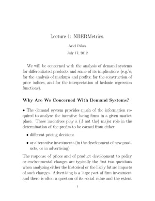
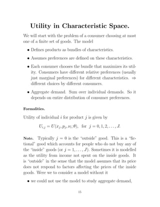
5. Digression; Aggregation and Simulation in Estima-
tion. Used for prediction by McFadden, Reid, Travilte , and
Johnson ( 1979, BART Project Report), and in estimation by
Pakes, 1986.
Though we often do not have information on which consumer
purchased what good, we do have the distribution of consumer
characteristics in the market of interest (e.g. the CPS). Let z
denote consumer characteristics, F (z) be their distribution, pj
be the price of the analyzed, p−j be the prices of competing
goods.
We have a model for individual utility given (z, pj , p−j ) which
depends on a parameter vector to be estimated (θ) and gener-
ates that indiviudal’s demand for good j,say q(z, pj , p−j ; θ).
Then aggregate demand is
D(pj , p−j ; F, θ) = z
q(z, pj , p−j ; θ)d F (z).
This may be hard to calculate exactly but it is easy enough to
simulate an estimate of it. Take ns random draws of z from
F (·), say (z1, . . . , zns), and define your estimate of D(pj , p−j ; F, θ)
to be ns
ˆ j , p−j ; F, θ) =
D(p q(zi, pj , p−j ; θ).
i=1
If E(·) provides the expectation and V ar(·) generates the vari-
ance from the simulation process
ˆ
E[D(pj , p−j ; F, θ)] = D(pj , p−j ; F, θ),
and
ˆ
V ar[D(pj , p−j ; F, θ)] = ns−1V ar(q(zi, pj , p−j ; θ)).
5

6. So our estimate is unbiased and can be made as precise as we
like by increasing ns.
Product space and heterogenous agents. We will fo-
cus on heterogenous agent models in characteristic space for the
reasons discussed below. However, at least in principle, demand
systems in characteristic space are approximations to product
space demand systems, and the approximations can be prob-
lematic1. On the other hand when it is feasible to use a product
space model there are good reasons to use heterogeneous agent
versions of it. This is because with heterogenous agents the
researhcer
• can combine data from different markets and/or time peri-
ods in a sensible way, and in so doing add the information
content of auxiliary data sets,
• and can get some idea of the entire distribution of responses.
The first point is important. Say we are interested in the im-
pact of price on demand. Micro studies typically show that the
price coefficient depends in an important way on income (or
some more inclusive measure of wealth); lower income people
care about price more. Consequently if the income distribution
varies across the markets studied, we should expect the price
coefficients to vary also, and if we did not allow for that it is
not clear what our estimate applies to.
1
I say in principle, because it may be impossible to add products every time a change in a
product’s characteristics occurs. In these cases researchers often aggregate products with slightly
different characteristics into one product, and allow for new products when characteristics change a
lot. So in effect they are using a “hybrid” model. It is also possible to explicitly introduces utility
as a function both products and characteristics; for a recent example see Dubois,Griffith, and Nevo
(2012, Working Paper.)
6

7. Further, even if we could chose markets with similar income
distributions, we typically would not want to. Markets with
similar characteristics should generate similar prices, so a data
set with similar income distributions would have little price vari-
ance to use in estimation.
In fact as the table below indicates, there is quite a bit of
variance in income distributions across local markets in the U.S.
The table gives means and standard deviations of the fraction of
the population in different income groups across U.S. counties.
The standard deviations are quite large, especially in the higher
income groups where most goods are directed.
Table I: Cross County Differences in Household Income∗
Income Fraction of U.S. Distribution of Fraction
Group Population in Over Counties
(thousands) Income Group Mean Std. Dev.
0-20 0.226 0.289 0.104
20-35 0.194 0.225 0.035
35-50 0.164 0.174 0.028
50-75 0.193 0.175 0.045
75-100 0.101 0.072 0.033
100-125 0.052 0.030 0.020
125-150 0.025 0.013 0.011
150-200 0.022 0.010 0.010
200 + 0.024 0.012 0.010
∗
From Pakes (2004, RIO) “Common Sense and Simplicity in Empirical Industrial
Organization”.
7

8. Multi-product Systems in Product
Space: Modelling Issues.
We need a model for the single agent and the remaining issues
with proudct space are embodied in that. They are
• The “too many parameter problem”. J goods implies on
the order of J 2 parameters (even from linear or log-linear
systems) and having on the order of 50 or more goods is
not unusual
• Can not analyze demand for new goods prior to product
introduction.
The Too Many Parameter Problem.
In order to make progress we have to aggregate over commodi-
ties. Two possibilities that do not help us are
• Hicks composite commodity theorem. pt = θtp0. Then
j j
demand is only a function of θ and p1, but we can not
study substitution patterns, just expansion along a path.
• Dixit-Stiglitz (or CES) preferences. Usually something like
( xρ)1/ρ. This rules out differential substitutions between
i
goods, so it rules out any analysis of competition between
goods. When we use it to analyze welfare, it is even more
restrictive than using simple logits (since they have an idi-
dosyncratic component), and you will see when we move to
welfare that the simple logit has a lot of problems.
8

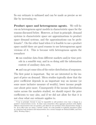
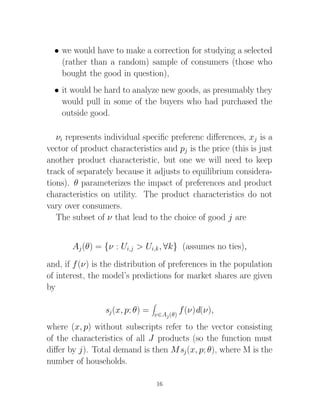
9. Gorman’s Polar Forms.
Basic idea of multilevel budgeting is
• First allocate expenditures to groups
• Then allocate expenditures within the group.
If we use a (log) linear system and there are J goods K groups
we get J 2/K + K 2 parameters vs J 2 + J (modulus other re-
strictions on utility surface). Still large. Moreover multilevel
budgeting can only be consistent if the utility function has two
peculiar properties
• We need to be able to order the bundles of commodities
within each group independent of the levels of purchases of
the goods outside the group, or weak separability
u(q1, ..., qJ ) = u[v1(q1), ..., vK (qK )].
where (q1, ..., qJ ) = (q1, ..., qK ). which means that for i
and j in different groups
∂qi ∂qi ∂qj
∝ × .
∂pj ∂x ∂x
(This implies that we determine all cross price elasticities
between goods in different groups by a number of parame-
ters equal to the number of groups).
• To be able to do the upper level allocation problem there
must be an aggregate quantity and price index for each
group which can be calculated without knowing the choices
within the groups.
9

10. These two requirements lead to Gorman’s (1968) polar forms
(these are if and only if conditions);
• Weak separability and constant budget shares within a
group (i.e. ηq,y = 1) (Weak separability is as above and
it implies that we can do the lower level allocation, con-
stant budget shares allows one to derive the price index for
the group without knowing the “income” allocated to the
group).
• Strong separability (additive), and budget shares need not
go through the origin.
These two restrictions are (approximately) implemented in the
Almost Ideal Demand Systems; see Deaton and Muelbauer
(1980)
Grouping Procedures More Generally.
If you actually consider the intuitive basis for Gorman’s condi-
tions for a given grouping, they often seem a priori unreason-
able. More generally, grouping is a movement to characteristics
models where we group on characteristics. There are problems
with it as we have to put products in mutually disjoint sets
(which can mean lots of sets), and we have to be extremely
careful when we “group” according to a continuous variable.
For example if you group on price and there is a demand side
residual correlated with price (a statement which we think is
almost always correct, see the next lecture) you will induce a
selection problem that is hard to handle. These problems disap-
pear when you move to characteristic space (unless you group
10

11. there also, like in Nested Logit, where they reappear). Empir-
ically when grouping procedures are used, the groups chosen
often depend on the topics of interest (which typically makes
different results on the same industry non-comparable).
11

12. An Intro to Characteristic Space.
Basic Idea. Products are just bundles of characteristics and
each individual’s demand is just a function of the characteristics
of the product (not all of which need be observed). This changes
the “space” in which we analyze demand with the following
consequences.
• The new space typically has a much smaller number of ob-
servable dimensions (the number of charactertistics) over
which we have preferences. This circumvents the “too many
parameter” problem. E.g. if we have k dimensions, and
the distribution of preferences over those dimensions was
say normal, then we would have k means and k(k + 1)/2
covariances, to estimate. If there were no unobserved char-
acteristics the k(1 + (k + 1)/2) parameters would suffice to
analyze own and cross price elasticities for all J goods, no
matter how large J is.
• Now if we have the demand system estimated, and we know
the proposed characteristics of a new good, we can, again
at least in principle, analyze what the demand for the new
good would be; at least conditional on the characteristics
of competing goods when the new good is introduced.
Historical Note. This basic idea first appeared in the de-
mand literature in Lancaster (1966, Journal of Political Econ-
omy), and in empirical work in McFadden (1973, “’Conditional
logit analysis of qualitative choice behavior’ in P. Zarembka,
(ed.), Frontiers in Econometrics). There was also an exten-
sive related literature on product placement in I.O. where some
12

13. authors worked with vertical(e.g. Shaked and Sutton) and some
with horizontal (e.g. Salop) characteristics. For more on this
see Anderson, De Palma and Thisse (and the reading list has
all these sites ).
Modern. Transfer all this into an empirically useable the-
ory of market demands and provide the necessary estimation
strategies. Greatly facilitated by modern computers.
Product space problems in characteristic space analysis. The
two problems that appear in product space re-appear in char-
acteristic space, but in a modified form that, at least to some
extent, can be dealt with.
• If there are lots of characteristics the too many parameter
problem re-appears and now we need data on all these char-
acteristics as well as price and quantity. Typically this is
more of a problem for consumer goods than producer goods
(which are often quite well defined by a small number of
characteristics). The “solution” to this problem will be to
introduce unobserved characteristics, and a way of dealing
with them. This will require a solution to an “endogeneity”
problem similar to the one you have seen in standard de-
mand and suppy analysis, as the unobserved characteristic
is expected to be correlated wth price.
• We might get a reasonable prediction for the demand for
a new good whose characteristics are similar (or are in the
span) of goods already marketed. However there is no in-
formation in the data on the demand for a characteristic
13

14. bundle that is in a totally new part of the characteristic
space. E.g. the closest thing to a laptop that had been
available before the laptop was a desktop. The desktop
had better screen resolution, more memory, and was faster.
Moreover laptops’ initial prices were higher than desktops;
so if we would have relied on demand and prices for desk-
tops to predict demand for laptops we would have predicted
zero demand.
There are other problems in characteristic space of varying im-
portance that we will get to, many of which are the subject of
current research. Indeed just as in any other part of empirical
economics these systems should be viewed as approximations to
more complex processes. One chooses the best approximation
to the problem at hand.
14

15. Utility in Characteristic Space.
We will start with the problem of a consumer choosing at most
one of a finite set of goods. The model
• Defines products as bundles of characteristics.
• Assumes preferences are defined on these characteristics.
• Each consumer chooses the bundle that maximizes its util-
ity. Consumers have different relative preferences (usually
just marginal preferences) for different characteristics. ⇒
different choices by different consumers.
• Aggregate demand. Sum over individual demands. So it
depends on entire distribution of consumer preferences.
Formalities.
Utility of individual i for product j is given by
Ui,j = U (xj , pj , νi; θ), for j = 0, 1, 2, . . . , J.
Note. Typically j = 0 is the “outside” good. This is a “fic-
tional” good which accounts for people who do not buy any of
the “inside” goods (or j = 1, . . . , J). Sometimes it is modelled
as the utility from income not spent on the inside goods. It
is “outside” in the sense that the model assumes that its price
does not respond to factors affecting the prices of the inside
goods. Were we to consider a model without it
• we could not use the model to study aggregate demand,
15

16. • we would have to make a correction for studying a selected
(rather than a random) sample of consumers (those who
bought the good in question),
• it would be hard to analyze new goods, as presumably they
would pull in some of the buyers who had purchased the
outside good.
νi represents individual specific preferenc differences, xj is a
vector of product characteristics and pj is the price (this is just
another product characteristic, but one we will need to keep
track of separately because it adjusts to equilibrium considera-
tions). θ parameterizes the impact of preferences and product
characteristics on utility. The product characteristics do not
vary over consumers.
The subset of ν that lead to the choice of good j are
Aj (θ) = {ν : Ui,j > Ui,k , ∀k} (assumes no ties),
and, if f (ν) is the distribution of preferences in the population
of interest, the model’s predictions for market shares are given
by
sj (x, p; θ) = ν∈Aj (θ)
f (ν)d(ν),
where (x, p) without subscripts refer to the vector consisting
of the characteristics of all J products (so the function must
differ by j). Total demand is then M sj (x, p; θ), where M is the
number of households.
16

17. Details.
Our utility functions are “cardinal”, i.e. the choices of each
individual are invariant to affine transformations, i.e.
1. multiplication of utility by a person specific positive con-
stant, and
2. addition to utility of any person specifc number.
This implies that we have two normalizations to make. In mod-
els where utility is (an individual specific) linear function of
product characteristics, the normalizations we usually make are
• normalize the value of the outside good to zero. Equivalent
to subtracting Ui,0 from all Ui,j .
• normalize the coefficient of one of the variables to one (in
the logit case this is generally the i.i.d error term; see be-
low).
The interpretation of the estimation results has to take these
normalizations into account; e.g. when we estimate utility for
choice j we are measuring the difference between its utility and
that for choice zero, and so on.
Simple Examples.
• Pure Horizontal. In the Hotelling story the product charac-
teristic is its location, person characteristic is its location.
With quadratic transportation costs we have
Ui,j = u + (yi − pj ) + θ(δj − νi)2.
17

18. Versions of this model have been used extensively by theo-
rists to gain intuition for product placement problems (see
the Tirole readings). There is only two product character-
istics in this model (price and product location), and the
coefficient of one (here price) is normalized to one. Every
consumer values a given location differently. When con-
sumers disagree on the relative values of a characteristic we
usually call the characteristic “horizontal”. Here there is
only one such characteristic (product location).
• Pure Vertical. Mussa-Rosen, Gabsewicz-Thisse, Shaked-
Sutton, Bresnahan. Two characteristics: quality and price,
and this time the normalization is on the quality coefficient
(or, equivalently, the inverse of the price coefficient). The
distinguishing feature here is that all consumers agree on
the ranking of the characteristic (quality) of the different
products. This defines a vertical characteristic.
Ui,j = u − νipj + δj , with νi > 0.
This is probably the most frequently used other model for
analyzing product placement (see also Tirole and the refer-
ences therein). When all consumers agree on the ranking of
the characteristic across products we (like quality here) we
call it a “vertical” characteristic. Price is usually considered
a vertical characteristic.
• “Logit”. Utiilty is mean quality plus idiosyncratic tastes
for a product.
Ui,j = δj + i,j .
18

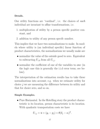
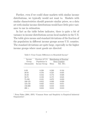
19. You have heard of the logit because it has tractible analytic
properties. In praticular if distributes i.i.d. (over both
products and individuals), and F ( ) = exp(−[exp(− )]),
then there is a closed, analytic form for both
– the probability of the maximum choice conditioned on
the vector of δ’s and
– the expected utility conditional on δ.
The closed form for the probability of choice eases esti-
mation, and the closed form for expected utility eases the
subsequent analysis of welfare. Further these are the only
known distributional assumption that has closed form ex-
pressions for these two magnitudes. For this reason it was
used extensively in empirical work (especially before com-
puters got good). Note that implicit in the distributional
assumption is an assumption on the distribution of tastes,
an assumption called the independence of irrelevant alter-
natives (or IIA) property. This is not very attractive for
reasons we review below.
The Need to Go to the Generalizations.
It is useful to see what the restrictions the simple forms of these
models imply, as they are the reasons we do not use them in
empirical work.
The vertical model. Ui,j = δj − νipj , where δj is the quality
of the good, and νi differs across individuals.
19

20. First, this specification implies that prices of goods must be
ordered by their qualities; if one good has less quality than
another but a higher price, no one would ever buy the lower
quality good. So we order the products by their quality, with
product J being the highest quality good. We can also order
individuals by their ν values; individuals with lower ν values
will buy higher priced, and hence higher quality, goods.
Now consider how demand responds to an increase in price of
good j. There will be some ν values that induce consumers that
would have been in good j to move to good j +1, the consumers
who were almost indifferent between these two goods. Similarly
some of the ν values would induce consumers who were at good
j to move to j − 1. However no consumer who choses any
other good would change their choice; if the other good was the
optimal choice before, it will certainly be optimal now.
So we have the implication that
• Cross price elasticities are only non-zero with neighboring
goods; with neighbors defined by prices, and
• Own price elasticities only depend on the density of the
distribution of consumers about the two indifference points.
Now consider a particular market, say the auto market. If we
line cars up by price we might find that a Ford Explorer (which
is an SUV) is the “neighbor” of a Mini Cooper S, with the Mini’s
neighbor being a GM SUV. The model would say that if the
Explorer’s price goes up none of the consumer’s who substitute
away from the Explorer would subsitute to the GM SUV, but
a lot would substitute to the Cooper S. Similarly the density of
20

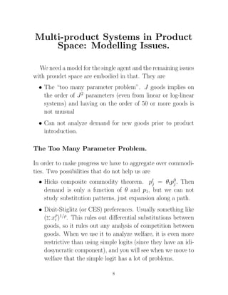
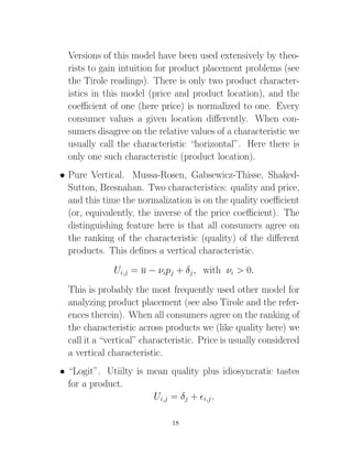
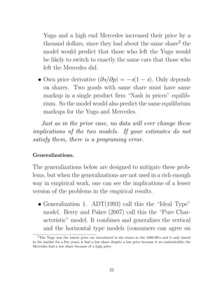
21. consumer’s often has little to do with what we think determines
price elasticities (and hence in a Nash pricing model, markups).
For example, we often think of symmetric or nearly symmetric
densities in which case low and high priced goods might have
the same densities about their indifference points, but we never
expect them to have the same elasticities or markups.
These problems will occur whenever the vertical model is
estimated; that is, if these properties are not generated by the
estimates, you have a computer programming error.
The Pure Logit. I.e; Ui,j = δj + i,j with independent over
products and agents. IIA problem. The distribution of a con-
sumer’s preferences over products other than the product it
bought, does not depend on the product if bought. Intuitively
this is problematic; we think that when a consumer switches out
of a car, say because of a price rise, the consumer will switch to
other cars with similar characteristics.
With the double exponential functional form for the distri-
bution it gives us an analytic form for the probabilities
exp[δj − pj ]
sj (θ) =
1 + q exp[δq − pq ]
1
s0(θ) =
1 + q exp[δq − pq ]
This implies the follwing.
• Cross price derivatives are sj sk . Two goods with the same
shares have the same cross price elasticities with any other
good regardless of that goods characteristics. So if both a
21

22. Yugo and a high end Mercedes increased their price by a
thouand dollars, since they had about the same share2 the
model would predict that those who left the Yugo would
be likely to switch to exactly the same cars that those who
left the Mercedes did.
• Own price derivative (∂s/∂p) = −s(1 − s). Only depends
on shares. Two goods with same share must have same
markup in a single product firm “Nash in prices” equilib-
rium. So the model would also predict the same equilibrium
markups for the Yugo and Mercedes.
Just as in the prior case, no data will ever change these
implications of the two models. If your estimates do not
satisfy them, there is a programing error.
Generalizations.
The generalizations below are designed to mitigate these prob-
lems, but when the generalizations are not used in a rich enough
way in empirical work, one can see the implications of a lesser
version of the problems in the empirical results.
• Generalization 1. ADT(1993) call this the “Ideal Type”
model. Berry and Pakes (2007) call this the “Pure Char-
acteristic” model. It combines and generalizes the vertical
and the horizontal type models (consumers can agree on
2
The Yugo was the lowest price car introduced in the states in the 1980-90’s and it only lasted
in the market for a few years; it had a low share despite a low price because it ws undersirable; the
Mercedes had a low share because of a high price
22

23. the ordering of some characteristics and not others).
Ui,j = f (νi, pj ) + xj,k νi,r θk,r ,
k r
where again we have distinguished price from the other
product characteristics as we often want to treat price some-
what differently. A special case of this (after appropriate
normalizations) is the “ideal type” model
Ui,j = f (νi, pj ) + δj + αk (xj,k − νi,k )2.
k
• Generalization 2. BLP(1995)
Ui,j = f (νi, pj ) + xj,k νr,k θk,r + i,j .
k
BLP vs The Pure Characteristic Model. The only difference
between BLP and the pure characteristic model is the addi-
tion of the logit errors (the i,j ) to the utility of each choice.
As a result, from the point of view of modelling shares, it can
be shown that the pure characteristics is a a limiting case of
BLP; but it is not a special case and the difference matters3. In
particular it can only be approached if parameters grow with-
out bound. This is a case computers have difficulty handling,
and Monte Carlo evidence indicates that when we use the BLP
specification to approximate a data set which abides by the pure
characteristic model, it can do poorly.
This could be problematic, because the logit errors are there
for computatinal convenience rather than for their likely ability
3
It is easiest to see this if you rewrite the BLP utility equation with a different normalization.
Instead of normalizing the coefficient of to one, let it be σ > 0. Now divide by σ . As σ → 0,
the shares from the pure characteristics model converge to those from BLP.
23

24. to mimic real-world phenomena. Disturbances in the utility are
usually thought of as emanating from either missing product
or missing consumer characteristics, and either of these would
generate correlation over products for a given individual. As
a result, we might like a BLP-type specification that nests the
pure-characteristic model.
When might the logit errors cause problems? In markets
with a lot of competing goods, the BLP specification does not
allow for cross-price elasticities which are too large. This is
because the independence of the logit errors implies that there
are always going to be some consumers who like each good a
lot more than other goods, and this bounds markups and cross
price-elasticities. There is also the question of the influence of
these errors on welfare estimates, which we will come back to
in another lecture.
These are reasons to prefer the pure characteristics model.
However, for reasons to be described below, it is harder (though
not impossible) to compute, and so far the recently introduced
computational techniques which you will be introduced to in
the subsequent lecture, have not helped much on this problem.
This is the reason that you have seen more of BLP than the
pure characteristic model. Despite this its intuitive appeal and
increased computer power have induced a number of papers us-
ing the pure characteristic model; often in markets where there
are one or two dominant vertical characteristics (like computer
chips, see Nosko, 2011). We come back to this in our discussion
of computation.
24