Download to read offline
![Variational Inequalities Approach To Supply Chain Network Equilibrium
DOI: 10.9790/5728-116495102 www.iosrjournals.org 102 | Page
References
[1]. Fisher M.L. What is the Right supply chain for your product? Harvard Business Review 75 (2 march – April) 105- 116 (1997).
[2]. Lee H. L and Belington C. The evolution of supply chain management models and practice at Hewlett – Packard interface (1995)
[3]. D. Kinderlehrerand G.Stampachia (1980) . An introduction to Variational Inequalities and their application, Academic press, New
York.
[4]. R .Anupindi and Y ,bassok (1996) Distribution channel ,information system and virtual centralized proceedings of the
manufacturing and services operation management of society conference 87-92.
[5]. Chopra. S Meindl P. (2003) . Supply chain management strategy, planning and operation 2nd
ed Prentice Hall.
[6]. Simchi – Levi, D , Designing and managing the supply chain concepts, strategies and case studies . New York (2002).
[7]. Cohen M.A mallikS . 1997 , Global supply chain , Research and application , production and operation management .193-210
[8]. Ducan Robert . The six rule of logistics strategy implementation London :PA consulting Group (2001)
[9]. Mahajan and G.V Ryzin( 2001). Inventory competition under dynamic consumer choice, operation Research .
[10]. Nagurney A. and D .Zhang (1996) projected dynamical systems and variational inequalities.](https://image.slidesharecdn.com/l0116495102-160129081342/75/Variational-Inequalities-Approach-to-Supply-Chain-Network-Equilibrium-8-2048.jpg)

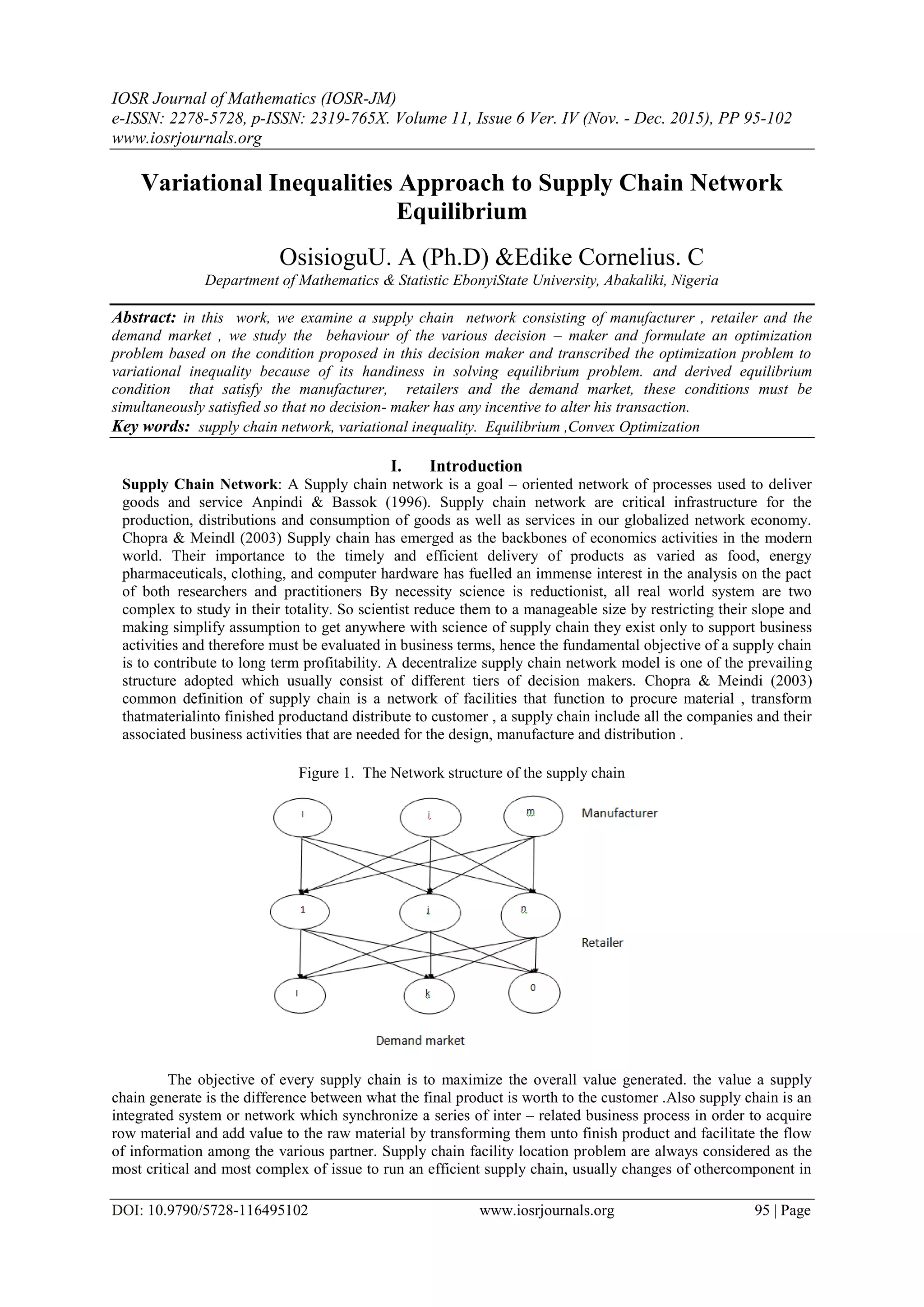
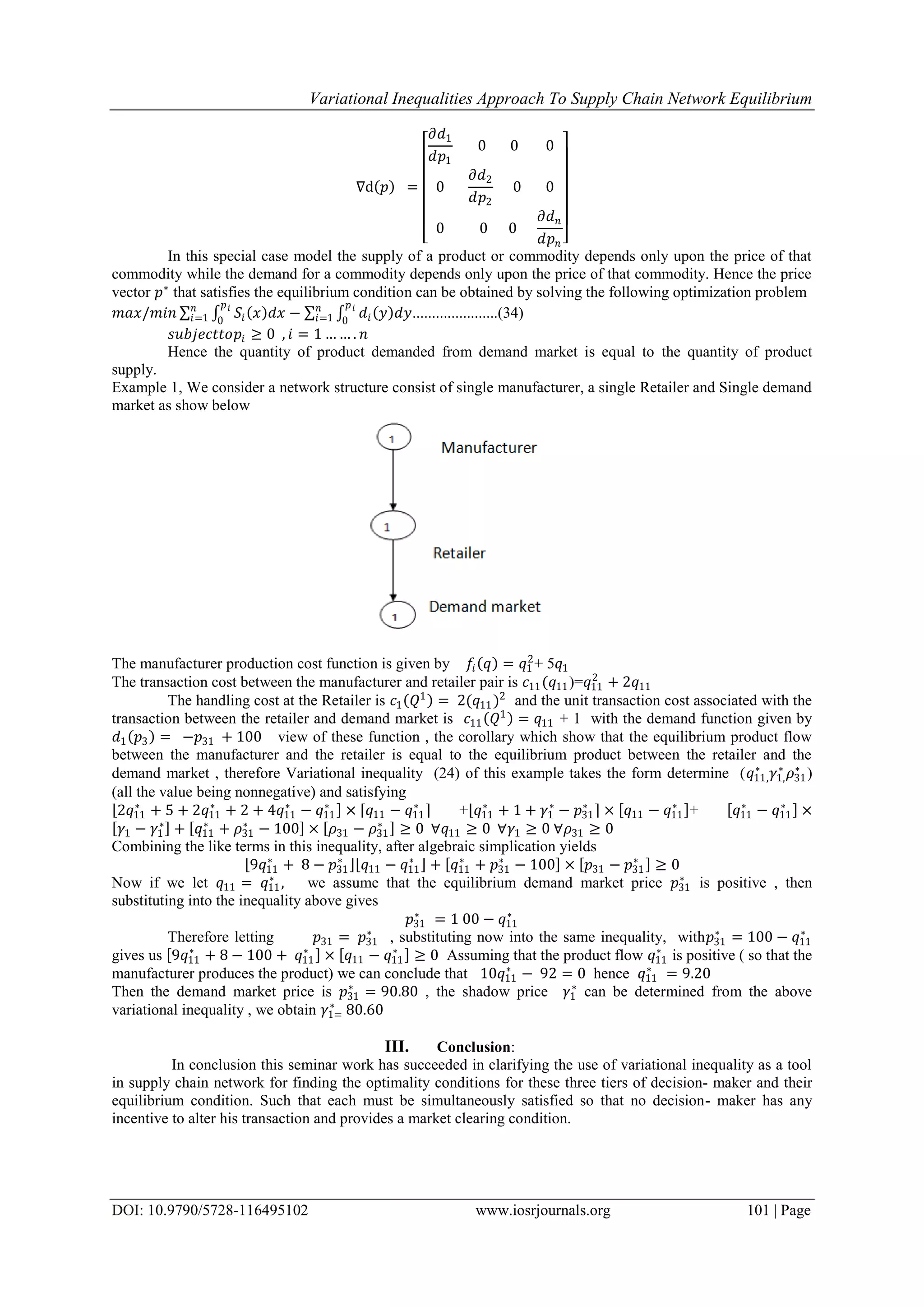
This document discusses a variational inequalities approach to establishing equilibrium in a supply chain network involving manufacturers, retailers, and demand markets. It formulates an optimization problem to analyze the behaviors of decision-makers within the supply chain and derives equilibrium conditions that must be satisfied to prevent any decision-maker from altering their transactions. The study contributes to understanding how to optimize supply chain operations and the interrelationships between various stakeholders.


