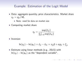
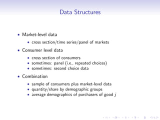
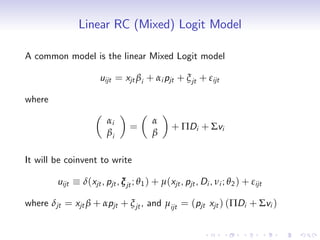
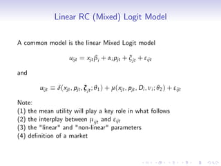
This document discusses methods for estimating static discrete choice models using market-level data rather than individual consumer data. It covers several key topics: 1) The types of market-level and consumer-level data that can be used. Market-level data is easier to obtain but poses challenges for identification and estimation. 2) A common linear random coefficients logit model framework. It includes observed and unobserved product characteristics as well as observed and unobserved consumer heterogeneity. 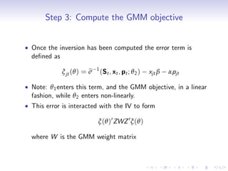3) The key challenges of estimating heterogeneity parameters without consumer-level data. It also discusses how to deal with potential endogeneity of unobserved product characteristics. 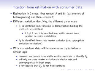4) The two-step estimation approach when consumer-level data is available, and

1. Estimation of Static Discrete Choice Models
Using Market Level Data
NBER Methods Lectures
Aviv Nevo
Northwestern University and NBER
July 2012

2. Data Structures
Market-level data
cross section/time series/panel of markets
Consumer level data
cross section of consumers
sometimes: panel (i.e., repeated choices)
sometimes: second choice data
Combination
sample of consumers plus market-level data
quantity/share by demographic groups
average demographics of purchasers of good j

3. Market-level Data
We see product-level quantity/market shares by "market"
Data include:
aggregate (market-level) quantity
prices/characteristics/advertising
de…nition of market size
distribution of demographics
sample of actual consumers
data to estimate a parametric distribution
Advantages:
easier to get
sample selection less of an issue
Disadvantages
estimation often harder and identi…cation less clear

4. Consumer-level Data
See match between consumers and their choices
Data include:
consumer choices (including choice of outside good)
prices/characteristics/advertising of all options
consumer demographics
Advantages:
impact of demographics
identi…cation and estimation
dynamics (especially if we have panel)
Disadvantages
harder/more costly to get
sample selection and reporting error

5. Review of the Model and Notation
Indirect utility function for the J inside goods
U (xjt , ξ jt , Ii pjt , Dit , νit ; θ ),
where
xjt – observed product characteristics
ξ jt – unobserved (by us) product characteristic
Dit – "observed" consumer demographics (e.g., income)
νit – unobserved consumer attributes
ξ jt will play an important role
realistic
will act as a "residual" (why don’ predicted shares …t exactly
t
– over…tting)
potentially implies endogeneity

6. Linear RC (Mixed) Logit Model
A common model is the linear Mixed Logit model
uijt = xjt βi + αi pjt + ξ jt + εijt
where
αi α
= + ΠDi + Σvi
βi β
It will be coinvent to write
uijt δ(xjt , pjt , ξ jt ; θ 1 ) + µ(xjt , pjt , Di , νi ; θ 2 ) + εijt
where δjt = xjt β + αpjt + ξ jt , and µijt = (pjt xjt ) (ΠDi + Σvi )

7. Linear RC (Mixed) Logit Model
A common model is the linear Mixed Logit model
uijt = xjt βi + αi pjt + ξ jt + εijt
and
uijt δ(xjt , pjt , ξ jt ; θ 1 ) + µ(xjt , pjt , Di , νi ; θ 2 ) + εijt
Note:
(1) the mean utility will play a key role in what follows
(2) the interplay between µijt and εijt
(3) the "linear" and "non-linear" parameters
(4) de…nition of a market

8. Key Challenges for Estimation
Recovering the non-linear parameters, which govern
heterogeneity, without observing consumer level data
The unobserved characteristic, ξ jt
a main di¤erence from early DC model (earlier models often
had option speci…c constant in consumer level models)
generates a potential for correlation with price (or other x’
s)
when constructing a counterfactual we will have to deal with
what happens to ξ jt
Consumer-level vs Market-level data
with consumer data, the …rst issue is less of a problem
the "endogeneity" problem can exist with both consumer and
market level data: a point often missed

9. What would we do if we had micro data?
Estimate in two steps.
First step, estimate (δ, θ 2 ) say by MLE
Pr(yit = j jDit , xt , pt , ξ t , θ ) = Pr(yit = j jDit , δ(xt , pt , ξ t , θ 1 ), xt , pt , θ
e.g., assume εijt is iid double exponential (Logit), and Σ = 0
expfδjt + (pjt xjt )ΠDi g
=
∑ J =0
k expfδkt + (pkt xkt )ΠDi g
Second step, recover θ 1
bjt = xjt β + αpjt + ξ
δ jt
ξ jt is the residual. If it is correlated with price (or x’ need
s)
IVs (or an assumption about the panel structure)

10. Intuition from estimation with consumer data
Estimation in 2 steps: …rst recover δ and θ 2 (parameters of
heterogeneity) and then recover θ 1
Di¤erent variation identfying the di¤erent parameters
θ 2 is identi…ed from variation in demographics holding the
level (i.e., δ) constant
If Σ 6= 0 then it is identi…ed from within market share
variation in choice probabilities
θ 1 is identi…ed from cross market variation (and appropriate
exclusion restrictions)
With market-level data will in some sense try to follow a
similar logic
however, we do not have within market variation to identify θ 2
will rely on cross market variation (in choice sets and
demographics) for both steps
a key issue is that ξ jt is not held constant

11. Estimation with market data: preliminaries
In principle, we could consider estimating θ by min the distance
between observed and predicted shares:
min kSt sj (xt , pt , θ )k
θ
Issues:
computation (all parameters enter non-linearly)
more importantly,
prices might be correlated with the ξ jt (“structural” error)
standard IV methods do not work

12. Inversion
Instead, follow estimation method proposed by Berry (1994)
and BLP (1995)
Key insight:
with ξ jt predicted shares can equal observed shares
Z
σj (δt , xt , pt ; θ 2 ) = 1 uijt uikt 8k 6= j dF (εit , Dit , νit ) = Sjt
under weak conditions this mapping can be inverted
1
δt = σ (St , xt , pt ; θ 2 )
the mean utility is linear in ξ jt ; thus, we can form linear
moment conditions
estimate parameters via GMM

13. Important (and often missed) point
IVs play dual role (recall 2 steps with consumer level data)
generate moment conditions to identify θ 2
deal with the correlation of prices and error
Even if prices are exogenous still need IVs
This last point is often missed
Why di¤erent than consumer-level data?
with aggregate data we only know the mean choice probability,
i.e., the market share
with consumer level data we know more moments of the
distribution of choice probabilities (holding ξ jt constant) :
these moments help identify the heterogeneity parameters

14. I will now go over the steps of the estimation
For now I assume that we have valid IVs
later we will discuss where these come from
I will follow the original BLP algorithm
I will discuss recently proposed alternatives later
I will also discuss results on the performance of the algorithm

15. The BLP Estimation Algorithm
1. Compute predicted shares: given δt and θ 2 compute
σj (δt , xt , pt ; θ 2 )
2. Inversion: given θ 2 search for δt that equates σj (δt , xt , pt ; θ 2 )
and the observed market shares
the search for δt will call the function computed in (1)
3. Use the computed δt to compute ξ jt and form the GMM
objective function (as a function of θ)
4. Search for the value of θ that minimizes the objective function

16. Example: Estimation of the Logit Model
Data: aggregate quantity, price characteristics. Market share
sjt = qjt /Mt
Note: need for data on market size
Computing market share
expfδjt g
sjt =
∑ J =0
k expfδkt g
Inversion
ln(sjt ) ln(s0t ) = δjt δ0t = xjt β + αpjt + ξ jt
Estimate using linear methods (e.g., 2SLS) with
ln(sjt ) ln(s0t ) as the "dependent variable".

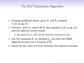
17. Step 1: Compute the market shares predicted by the model
Given δt and θ 2 (and the data) compute
Z
σj (δt , xt , pt ; θ 2 ) = 1 [uijt uikt 8k 6= j ] dF (εit , Dit , νit )
For some models this can be done analytically (e.g., Logit,
Nested Logit and a few others)
Generally the integral is computed numerically
A common way to do this is via simulation
1 ns
expfδjt + (pjt xjt )(ΠDi + Σvi )g
e
σj (δt , x t , p t , F ns ; θ 2 ) =
ns ∑ 1 + ∑J expfδkt + (pkt xkt )(ΠDi + Σ
i =1 k =1
where vi and Di , i = 1, ..., ns are draws from Fv (v ) and
FD ( D ) ,
Note:
the ε’ are integrated analytically
s
other simulators (importance sampling, Halton seq)
integral can be approximated in other ways (e.g., quadrature)

18. Step 2: Invert the shares to get mean utilities
Given θ 2 , for each market compute mean utility, δt , that
equates the market shares computed in Step 1 to observed
shares by solving
e
σ(δt , xt , pt , Fns ; θ 2 ) = St
For some model (e.g., Logit and Nested Logit) this inversion
can be computed analytically.
Generally solved using a contraction mapping for each market
δh +1 = δh + ln(St )
t t ln(σ(δh , xt , pt , Fns ; θ 2 ) h = 0, ..., H,
e t
where H is the smallest integer such that δH
t δH
t
1
<ρ
δH is the approximation to δt
t
Choosing a high tolerance level, ρ, is crucial (at least 10 12 )

19. Step 3: Compute the GMM objective
Once the inversion has been computed the error term is
de…ned as
1
e
ξ jt (θ ) = σ (St , xt , pt ; θ 2 ) xjt β αpjt
Note: θ 1 enters this term, and the GMM objective, in a linear
fashion, while θ 2 enters non-linearly.
This error is interacted with the IV to form
ξ (θ )0 ZWZ 0 ξ (θ )
where W is the GMM weight matrix

20. Step 4: Search for the parameters that maximize the
objective
In general, the search is non-linear
It can be simpli…ed in two ways.
“concentrate out” the linear parameters and limit search to θ 2
use the Implicit Function Theorem to compute the analytic
gradient and use it to aid the search
Still highly non-linear so much care should be taken:
start search from di¤erent starting points
use di¤erent optimizers

21. Identi…cation
Ideal experiment: randomly vary prices, characteristics and
availability of products, and see where consumers switch (i.e.,
shares of which products respond)
In practice we will use IVs that try to mimic this ideal
experiment
Next lecture we will see examples
Is there "enough" variation to identify substitution?
Solutions:
supply information (BLP)
many markets (Nevo)
add micro information (Petrin, MicroBLP)
For further discussion and proofs (in NP case) see Haile and
Berry

22. The Limit Distribution for the Parameter Estimates
Can be obtained in a similar way to any GMM estimator
With one cross section of observations is
J 1
(Γ0 Γ) 1 0
Γ V0 Γ ( Γ 0 Γ ) 1
where
Γ – derivative of the expectation of the moments wrt
parameters
V0 – variance-covariance of those moments evaluated
V0 has (at least) two orthogonal sources of randomness
randomness generated by random draws on ξ
variance generated by simulation draws.
in samples based on a small set of consumers: randomness in
sample
Berry Linton and Pakes, (2004 RESTUD): last 2 components
likely to be very large if market shares are small.
A separate issue: limit in J or in T
in large part depends on the data

23. Challenges
Knittel and Metaxoglou found that di¤erent optimizers give
di¤erent results and are sensitive to starting values
Some have used these results to argue against the use of the
model
Note, that its unlikely that a researcher will mimic the KM
exercise
start from one starting point and not check others
some of the algorithms they use are not very good and rarely
used
It ends up that much (but not all!) of their results go away if
use tight tolerance in inversion (10 12 )
proper code
reasonable optimizers
This is an important warning about the challenges of NL
estimation

24. MPEC
Judd and Su, and Dube, Fox and Su, advocate the use of
MPEC algorithm instead of the Nested …xed point
The basic idea: maximize the GMM objective function subject
to the "equilibrium" constraints (i.e., that the predicted
shares equal the observed shares)
Avoids the need to perform the inversion at each and every
iteration of the search
performing the inversion for values of the parameters far from
the truth can be quite costly
The problem to solve can be quite large, but e¢ cient
optimzers (e.g., Knitro) can solve it e¤ectively.
DFS report signi…cant speed improvements

25. MPEC (cont)
Formally
min ξ 0 ZWZ0 ξ
θ,ξ
subject to e
σ (ξ; x, p, Fns , θ ) = S
Note
the min is over both θ and ξ: a much higher dimension search
ξ is a vector of parameters, and unlike before it is not a
function of θ
avoid the need for an inversion: equilibrium constraint only
holds at the optimum
in principle, should yield the same solution as the nested …xed
point
Many bells and whistles that I will skip

26. ABLP
Lee (2011) builds on some of the ideas proposed in dynamic
choice to propose what he calls Approximate BLP
The basic idea
Start with a guess to ξ, denoted ξ 0 , and use it to compute a
…rst order Taylor approximation to σ(ξ t , xt , pt ; θ ) given by
∂ ln s (ξ 0 ; θ )
ln s (ξ t ; θ ) ln s A (ξ t ; θ ) ln s (ξ 0 ; θ ) +
t 0
t
(ξ t ξ0 )
t
ln ξ t
From ln St = ln s A (ξ t ; θ ) we get
" # 1
∂ ln s (ξ 0 ; θ )
ξt = Φt ( ξ 0 , θ )
t ξ0 +
t 0
t
(ln St ln s (ξ 0 ; θ ))
t
ln ξ t
Use this approximation for estimation
min Φ(ξ 0 , θ )0 ZWZ0 Φ(ξ 0 , θ )
θ

27. ABLP (cont)
Nest this idea into K-step procedure
Step 1: Obtain new GMM estimate
θ K = arg min Φ(ξ K 1
, θ )0 ZWZ0 Φ(ξ K 1
, θ)
θ
Step 2: Update ξ
ξ K = Φ(ξ K
t
1
, θK )
Repeat until convergence
Like MPEC avoids inversion at each stage, but has low
dimensional search
Lee reports signi…cant improvements over MPEC
Disclaimer: still a WP and has not been signi…cantly tested

28. Comparing the methods
Patel (2012, chapter 2 NWU thesis) compared the 3 methods

29. Comparing the methods
Word of caution: MPEC results can probably be signi…cantly
improved with better implementation
This is just an example of what one might expect if asking a
(good) RA to program these methods