The document discusses the keynesian model of income determination. It introduces concepts like aggregate demand, consumption function, planned investment, government purchases, net exports, and equilibrium income. Equilibrium income is where aggregate demand equals output and income. A change in autonomous spending will lead to a multiplied change in equilibrium income due to the income multiplier effect. The model can also take into account aspects like an open economy and the government sector.
Introduction to the Simple Keynesian Model focusing on Income Determination, outlining key components such as Consumption Function, Investment, Government Purchases, and Net Exports.
Explains the determinants of Equilibrium Output, showcasing Aggregate Demand (AD) and its relation with actual output and equilibrium levels.
Describes the Consumption Function, emphasizing the relationship between income and consumption, including the Marginal Propensity to Consume (MPC).
Derives the Savings Function, discussing the relationship between income and savings, and introducing constants for planned investment and government purchases.
Analyzes Equilibrium Income through Aggregate Demand, explaining inventory effects on production and income levels.
Derives equations to establish the equilibrium income levels depending on autonomous spending components.
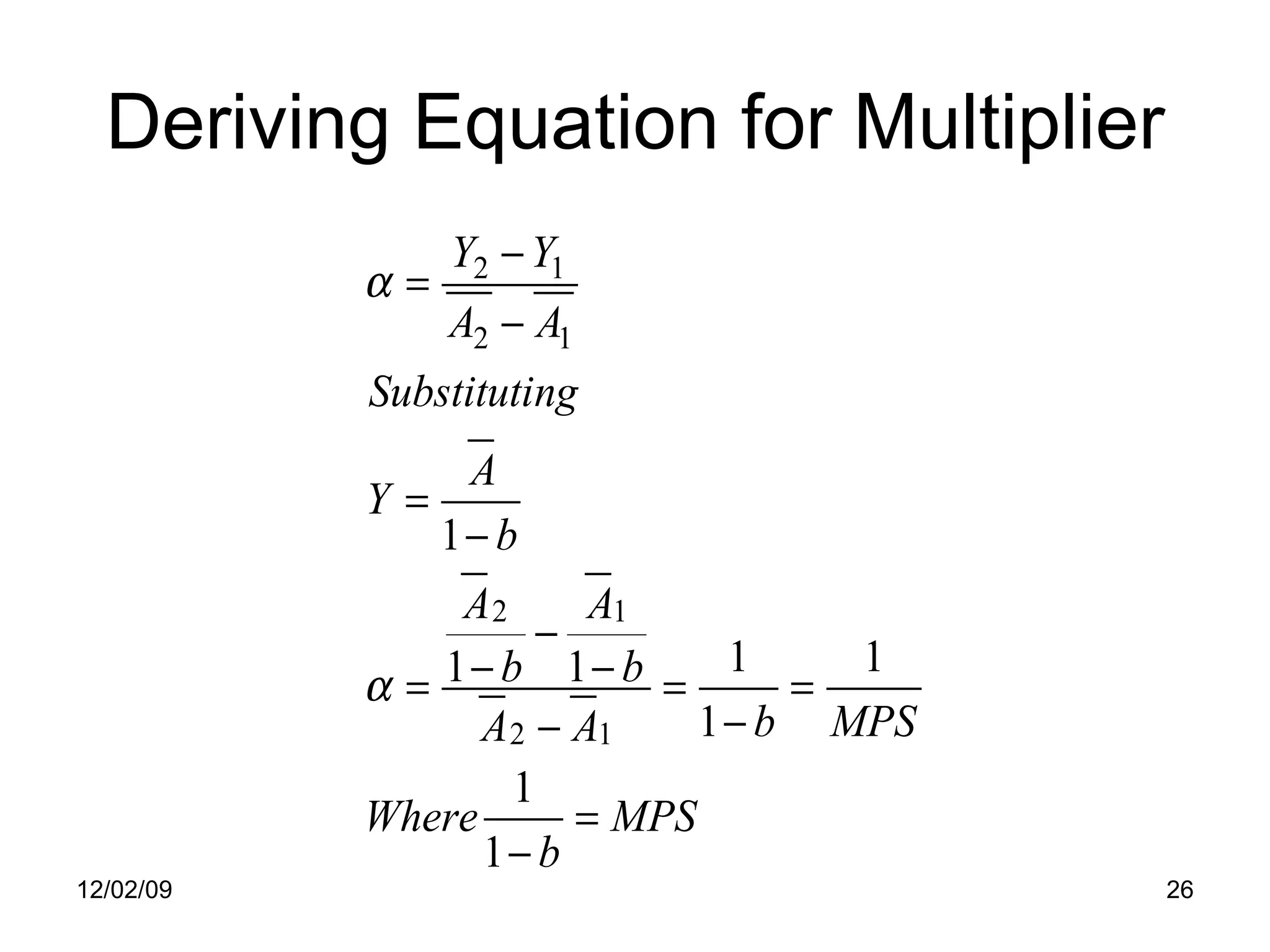
Explains the Multiplier effect, relating changes in equilibrium income to changes in autonomous spending, and discussing the roles of MPC and MPS.
Defines key concepts such as Disposable Income and Budget Surplus within the government sector influencing the economy.
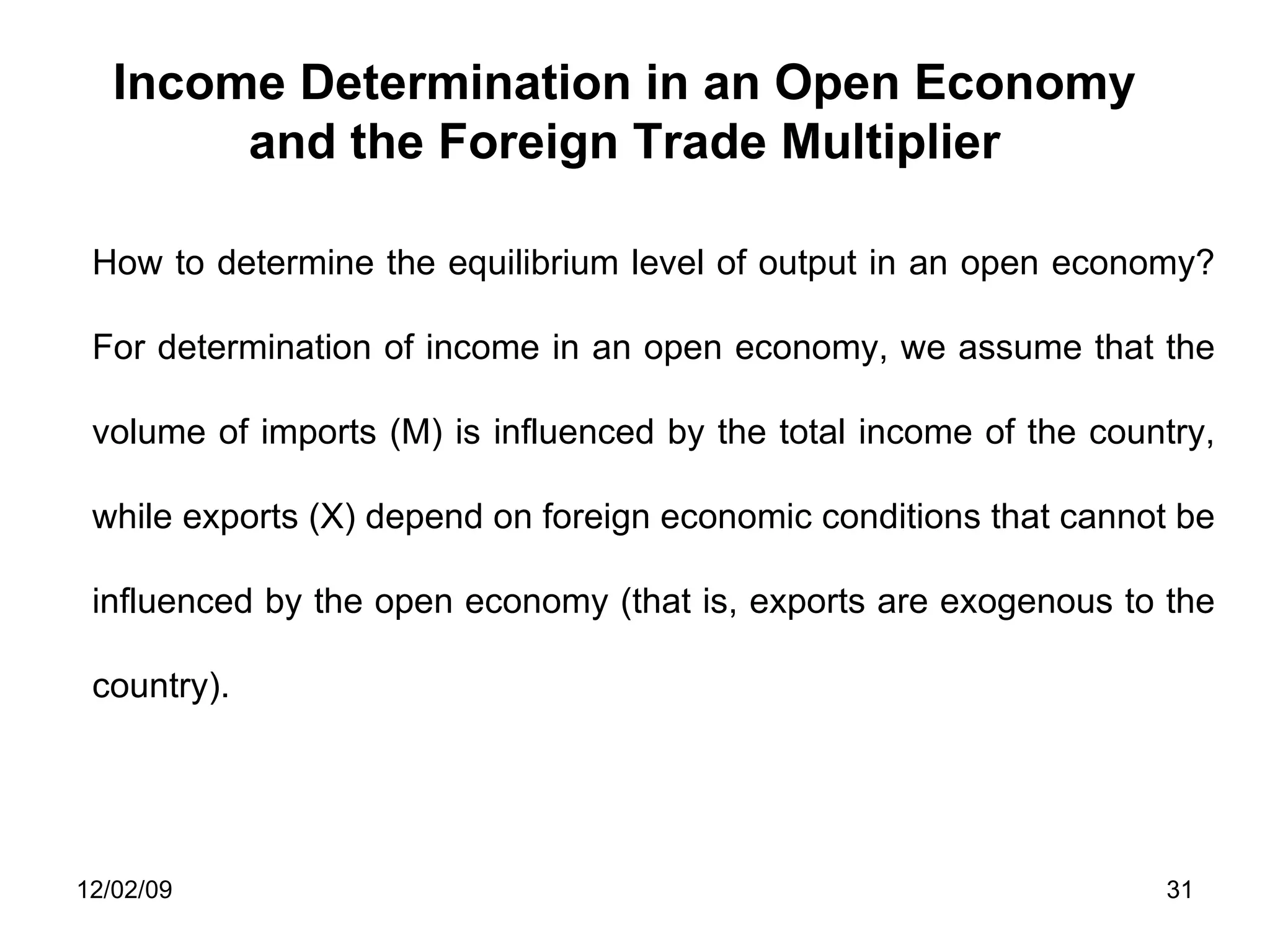
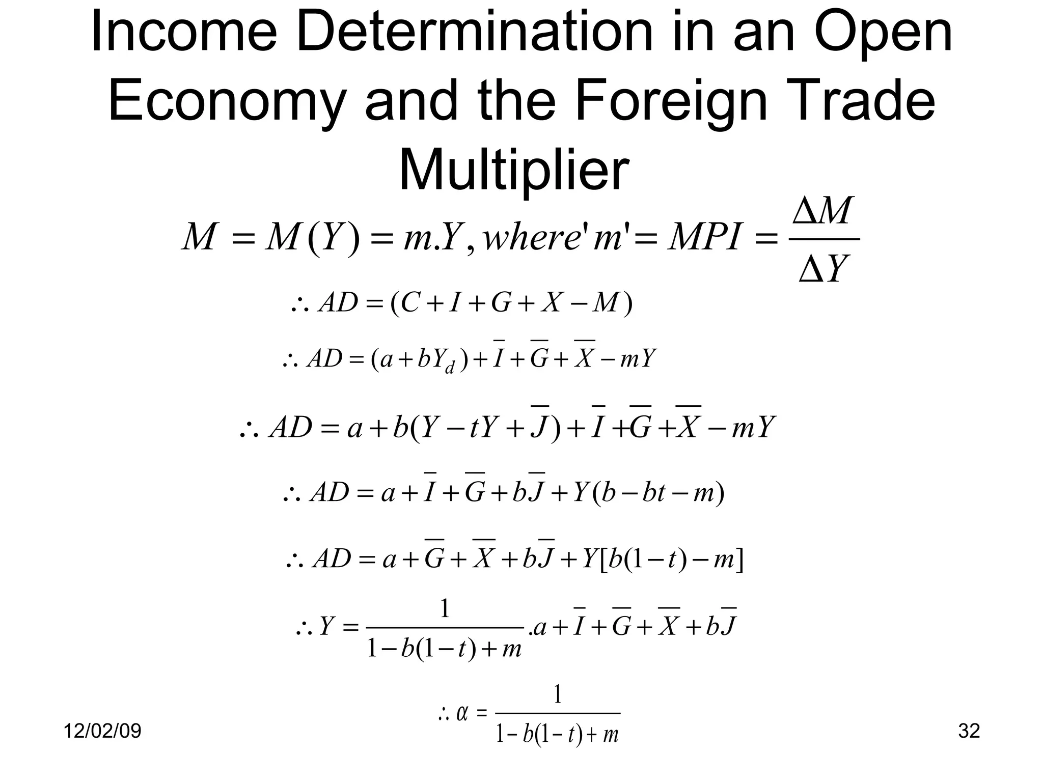
Examines how income determination occurs in an open economy, influenced by exports, imports, and foreign economic conditions.
Session Outline ConsumptionFunction Planned Investment (I), Government Purchases (G) and Net Exports (NX) Equilibrium Income Multiplier Income Determination in an Open Economy and the Foreign Trade Multiplier 06/07/09
3.
Introduction Full employmentlevel is one of the many possible states of the economy i.e., it need not be automatically at this state. The model focuses only on the goods market and the influence of money market on the goods market is completely ignored. Key assumptions. Prices remain constant Firms are able to sell any amount of output at given level of prices (that is, the aggregate supply curve is perfectly elastic) 06/07/09
4.
Determination of EquilibriumOutput Aggregate demand (AD) = total goods demanded in an economy. AD = C + I + G + NX 06/07/09
5.
Equilibrium Output Equilibriumoutput is the output level at which the quantity of output produced is equal to quantity of output demanded. At any output level, Y, is equal to C + I + G + NX. Does it mean all output levels are equilibrium output levels? The answer is ‘No’. 06/07/09
6.
Equilibrium Output Theconcept of aggregate demand, AD is ‘ex-ante’, national income accounts are all in the ‘ex-post’ sense. In other words, aggregate demand refers to the total goods and services that people want to buy, while national income refers to the total goods and services that are actually bought. 06/07/09
7.
Equilibrium Output Desiredaggregate demand may not be equal to actual output at all times. Equilibrium level of output refers to the output at which total desired spending on goods and services (desired aggregate demand) is equal to the actual level of output (Y). 06/07/09
8.
Determination of EquilibriumOutput Aggregate Demand (AD): AD = C + I + G + NX Equilibrium Output: Y = AD Or, Y = C + I + G + NX 06/07/09
9.
Consumption Function Consumptionexpenditure (C) is one of the important components of aggregate demand. Although many factors influence the consumption expenditure, income (Y) is considered to be the most important influencing factor. The relationship between consumption and income can be described using consumption function, C = f(Y). 06/07/09
10.
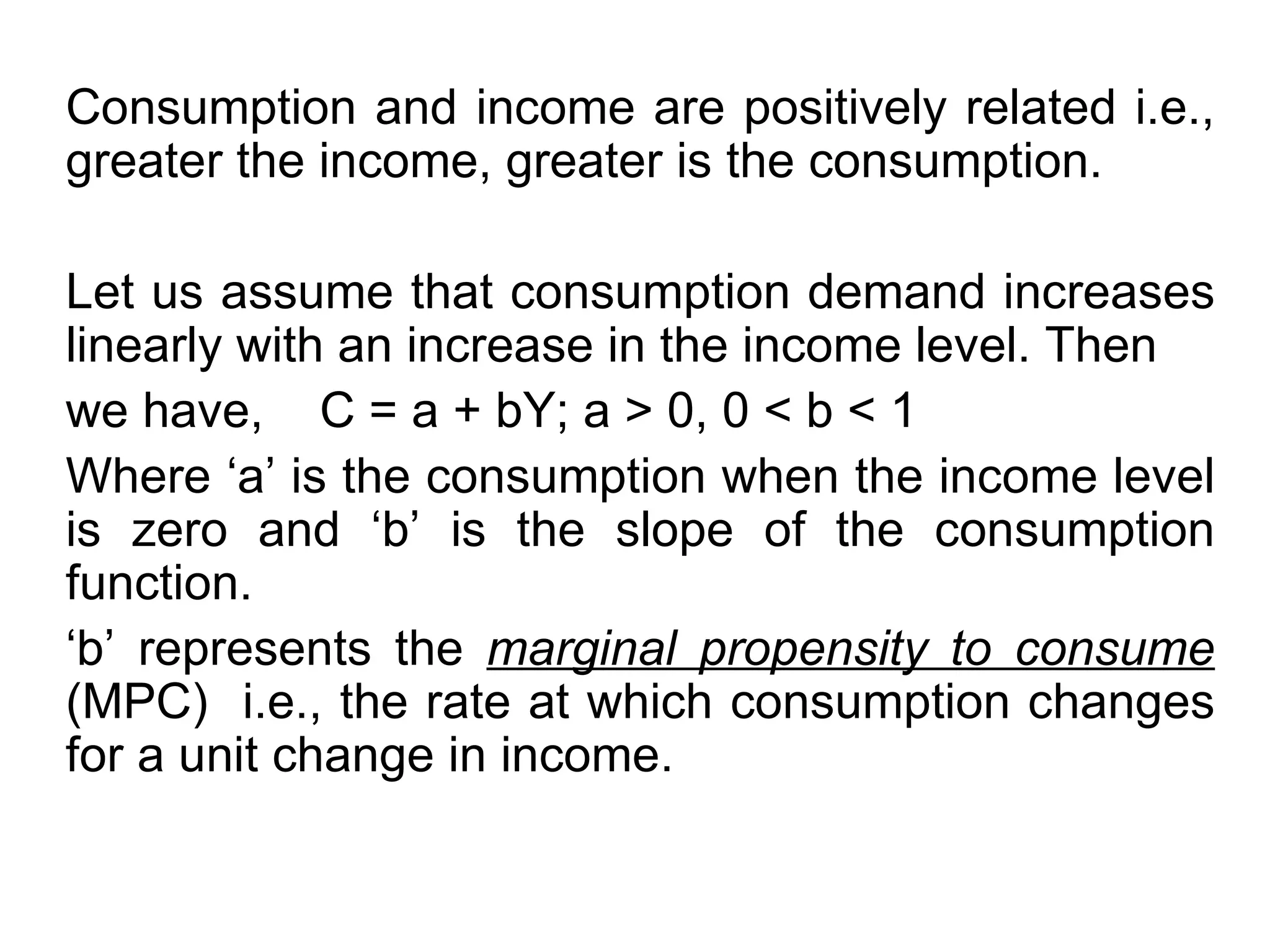
Consumption and incomeare positively related i.e., greater the income, greater is the consumption. Let us assume that consumption demand increases linearly with an increase in the income level. Then we have, C = a + bY; a > 0, 0 < b < 1 Where ‘a’ is the consumption when the income level is zero and ‘b’ is the slope of the consumption function. ‘ b’ represents the marginal propensity to consume (MPC) i.e., the rate at which consumption changes for a unit change in income.
11.
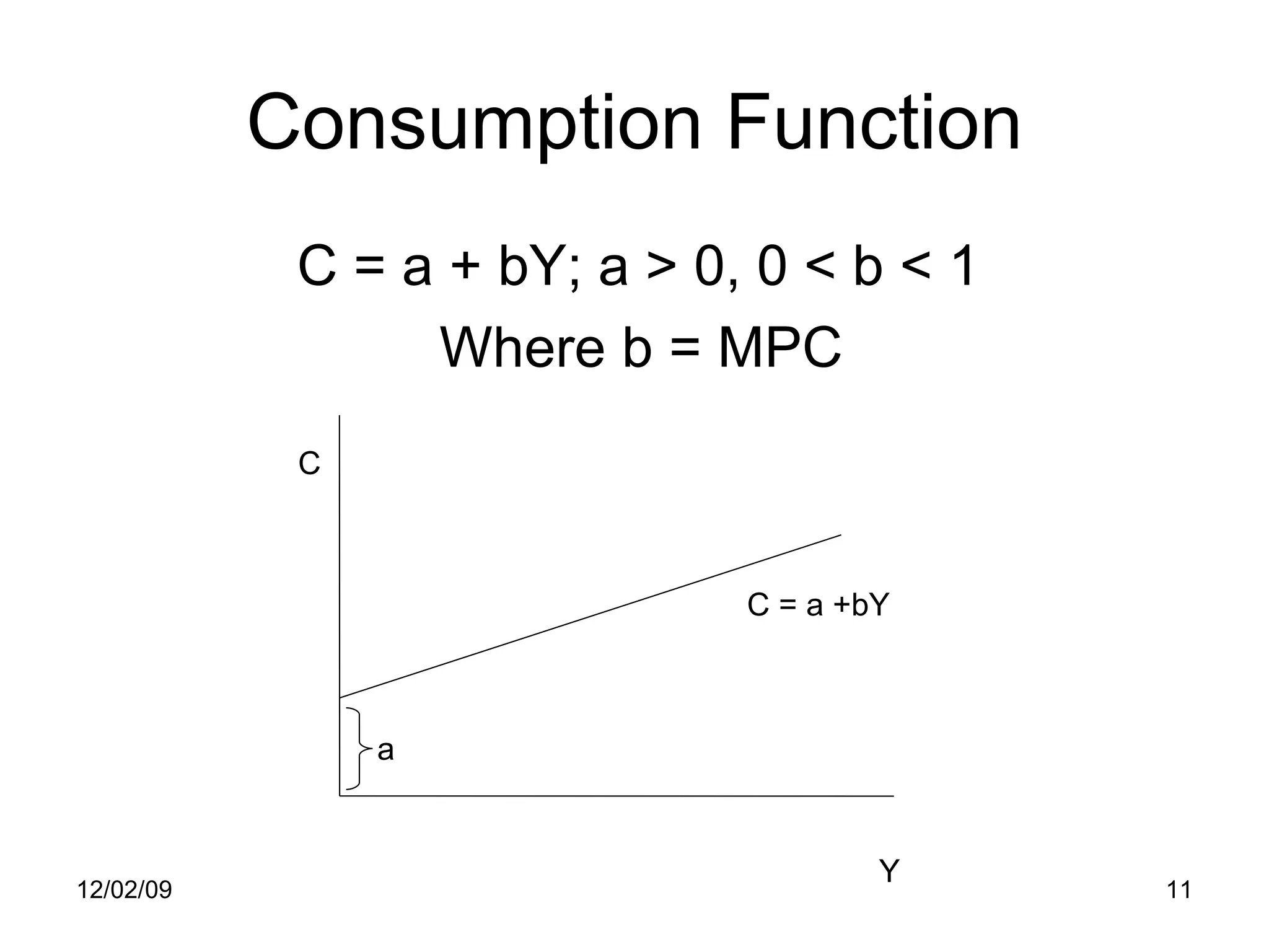
Consumption Function C = a + bY; a > 0, 0 < b < 1 Where b = MPC 06/07/09 C = a +bY a C Y
12.
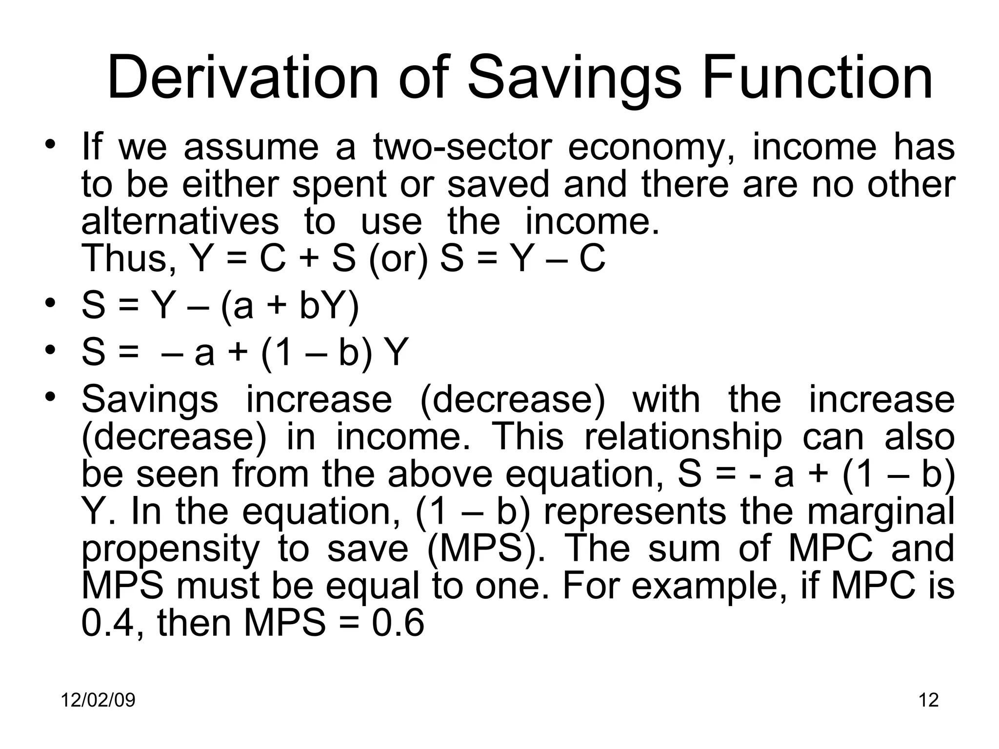
Derivation of SavingsFunction If we assume a two-sector economy, income has to be either spent or saved and there are no other alternatives to use the income. Thus, Y = C + S (or) S = Y – C S = Y – (a + bY) S = – a + (1 – b) Y Savings increase (decrease) with the increase (decrease) in income. This relationship can also be seen from the above equation, S = - a + (1 – b) Y. In the equation, (1 – b) represents the marginal propensity to save (MPS). The sum of MPC and MPS must be equal to one. For example, if MPC is 0.4, then MPS = 0.6 06/07/09
13.
Savings Function Y= C + S S = Y – C S = Y – C = Y – a – bY = - a + (1 – b)Y Where b = MPC 06/07/09
14.
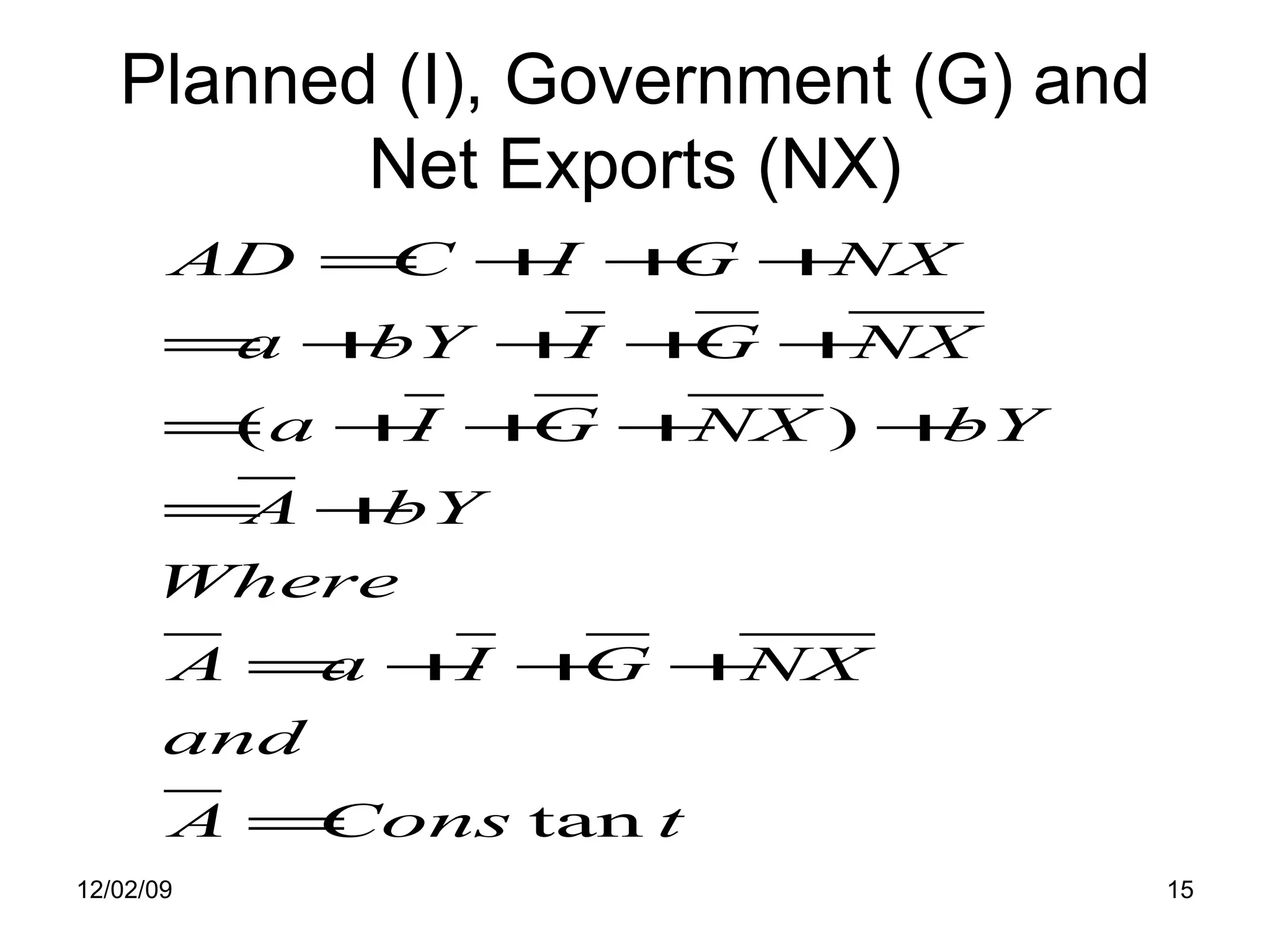
Planned Investment (I),Government Purchases (G) and Net Exports (NX) For deriving consumption function, we assume that other components of aggregate demand I, G and NX are constant and are independent of the income level. Let the constant levels of investment, government purchases and net exports be represented by I , G and NX respectively. 06/07/09
Planned Investment (I),Government Purchases (G) and Net Exports (NX) 06/07/09 C = a +bY AD = +bY Y AD a
17.
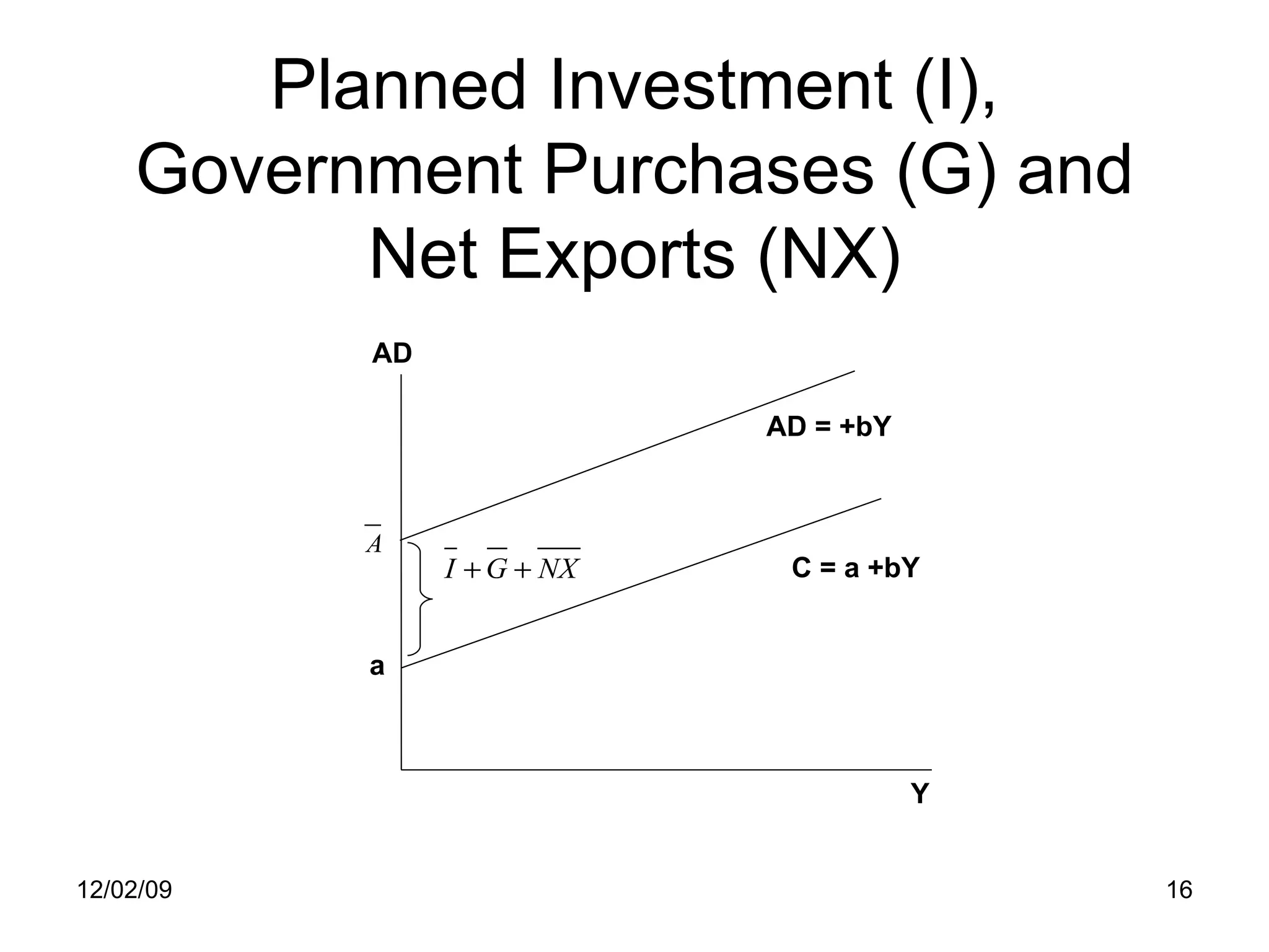
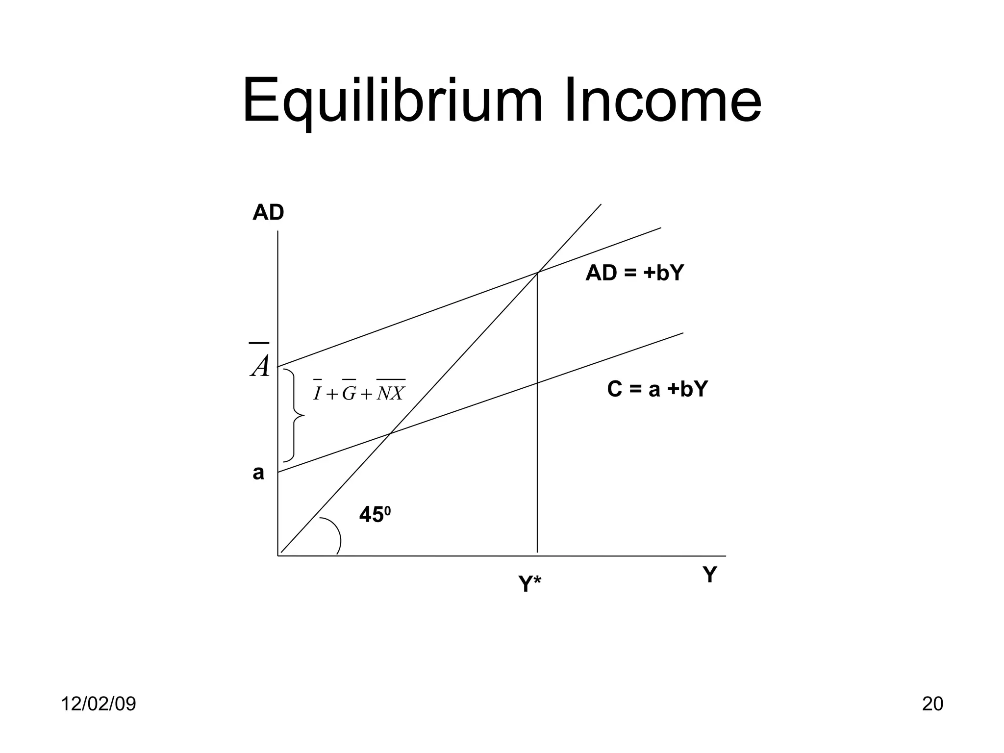
In the figure,we have shown consumption function and the aggregate demand function. The parallel line above the consumption function is the AD line. Part of the aggregate demand, i.e. is autonomous and is independent to the income level, while remaining part ‘bY’ is dependent on income and output. 06/07/09
18.
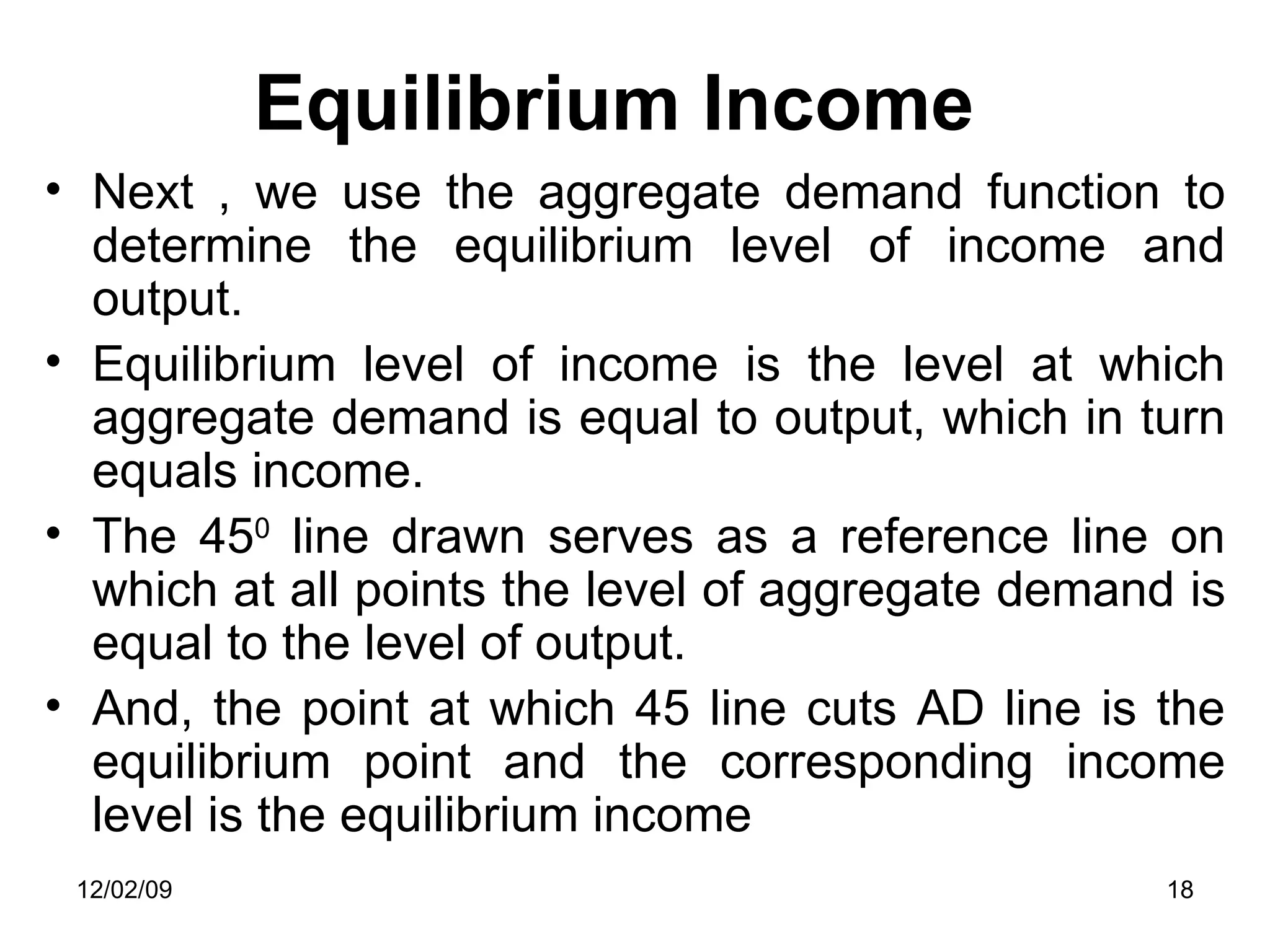
Equilibrium Income Next, we use the aggregate demand function to determine the equilibrium level of income and output. Equilibrium level of income is the level at which aggregate demand is equal to output, which in turn equals income. The 45 0 line drawn serves as a reference line on which at all points the level of aggregate demand is equal to the level of output. And, the point at which 45 line cuts AD line is the equilibrium point and the corresponding income level is the equilibrium income 06/07/09
19.
At output levelsbelow Y, aggregate demand exceeds output. Consequently, the level of inventory with firms decreases. This unintended (undesired) decline in inventories makes firms to increase their production, resulting in increase in income levels. Conversely, at output levels above Y, the output exceeds aggregate demand causing increase in level of inventories. This unintended increase in inventories makes firms to cut their production. 06/07/09
From the aboveformula, we know that larger the autonomous components (for a given b), the higher is the equilibrium level of income. Similarly, if b (slope of the AD curve) is less, then higher is the equilibrium level of income. 06/07/09
23.
Multiplier Multiplier refersto a multiple by which equilibrium income changes for a unit change in autonomous spending. Put differently, multiplier refers to the rate at which the level of equilibrium income increases (decreases) for a unit increase (decrease) in autonomous spending. The multiplier is denoted by . 06/07/09
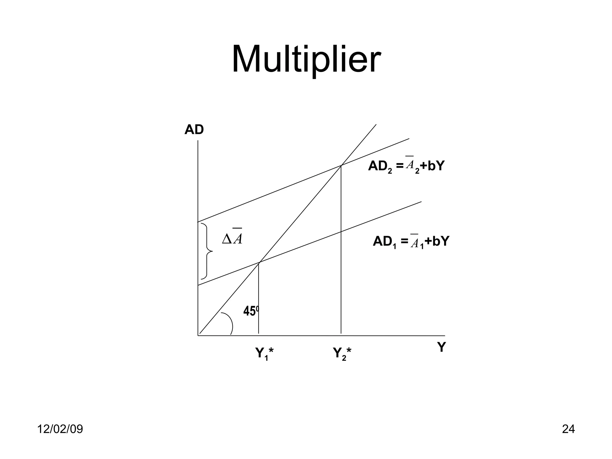
From the abovefigure it is clear that for a change in autonomous expenditure (∆A), there would be a greater change in equilibrium income (Y), because of operation of multiplier. 06/07/09
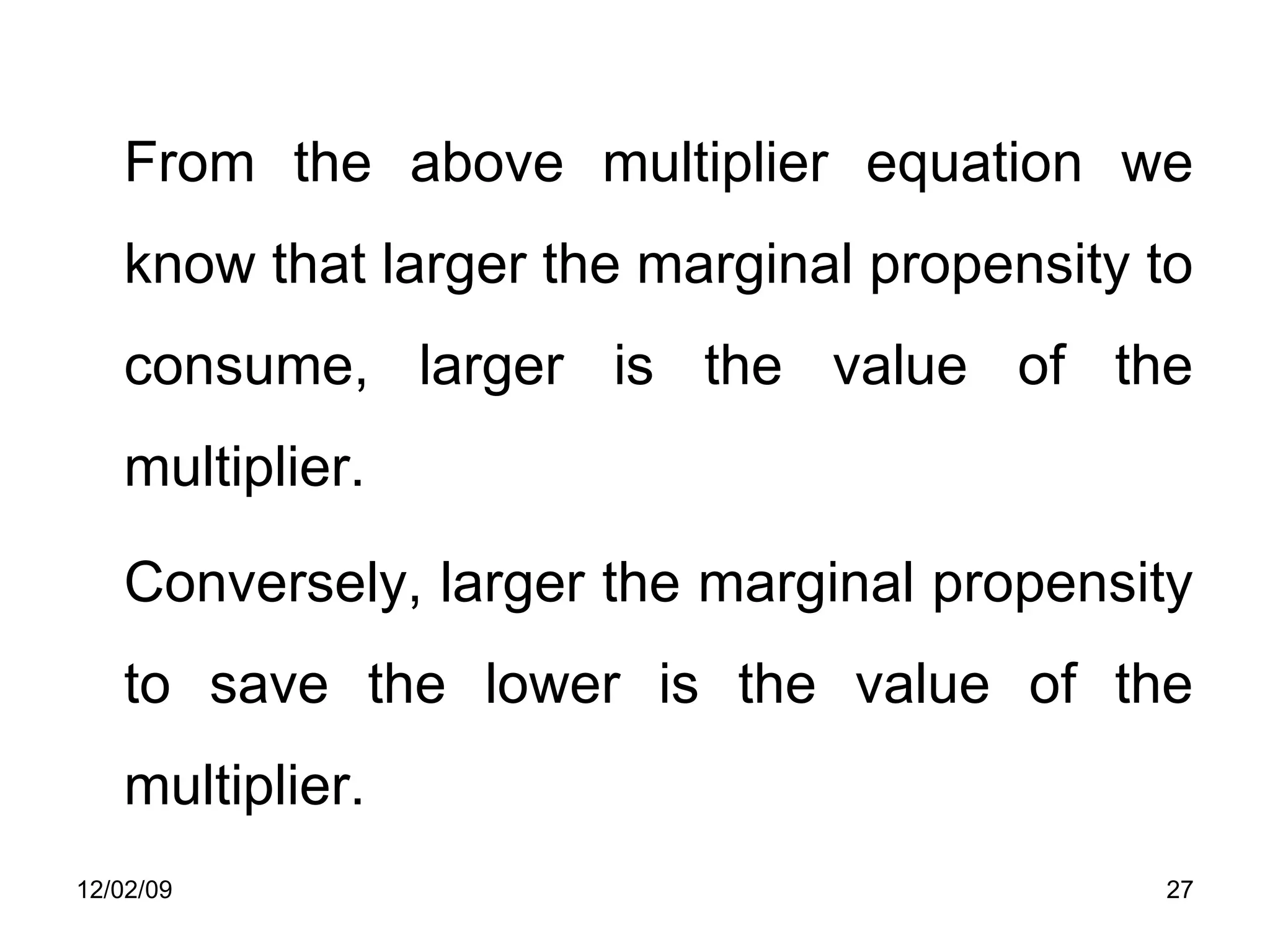
From the abovemultiplier equation we know that larger the marginal propensity to consume, larger is the value of the multiplier. Conversely, larger the marginal propensity to save the lower is the value of the multiplier. 06/07/09
28.
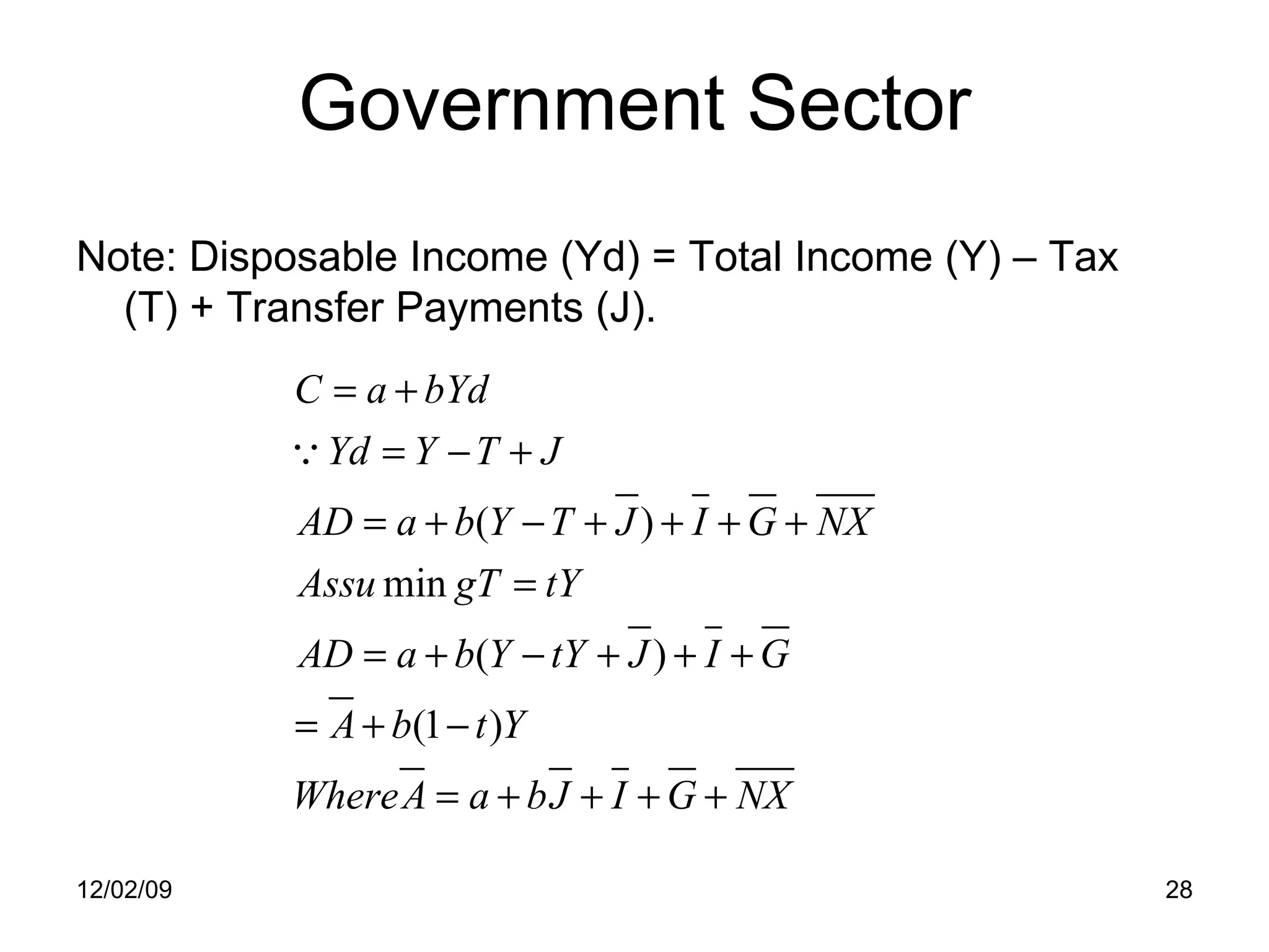
Government Sector Note:Disposable Income (Yd) = Total Income (Y) – Tax (T) + Transfer Payments (J). 06/07/09
The Budget BudgetSurplus (BS) = Tax Revenue (T) – Government Expenditure (G) – Transfer Payments (J) 06/07/09
31.
Income Determination inan Open Economy and the Foreign Trade Multiplier How to determine the equilibrium level of output in an open economy? For determination of income in an open economy, we assume that the volume of imports (M) is influenced by the total income of the country, while exports (X) depend on foreign economic conditions that cannot be influenced by the open economy (that is, exports are exogenous to the country). 06/07/09