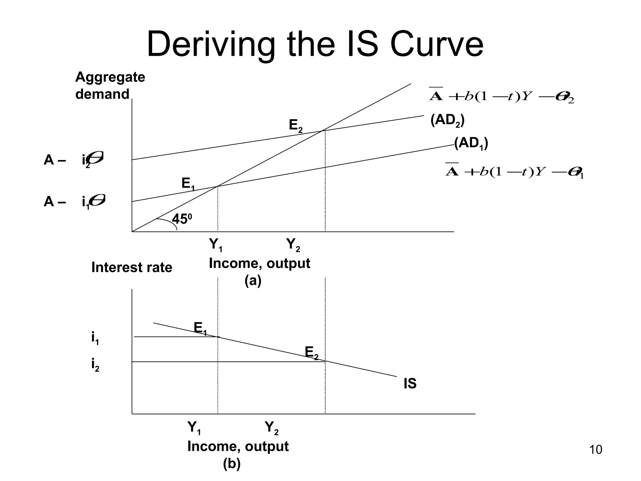
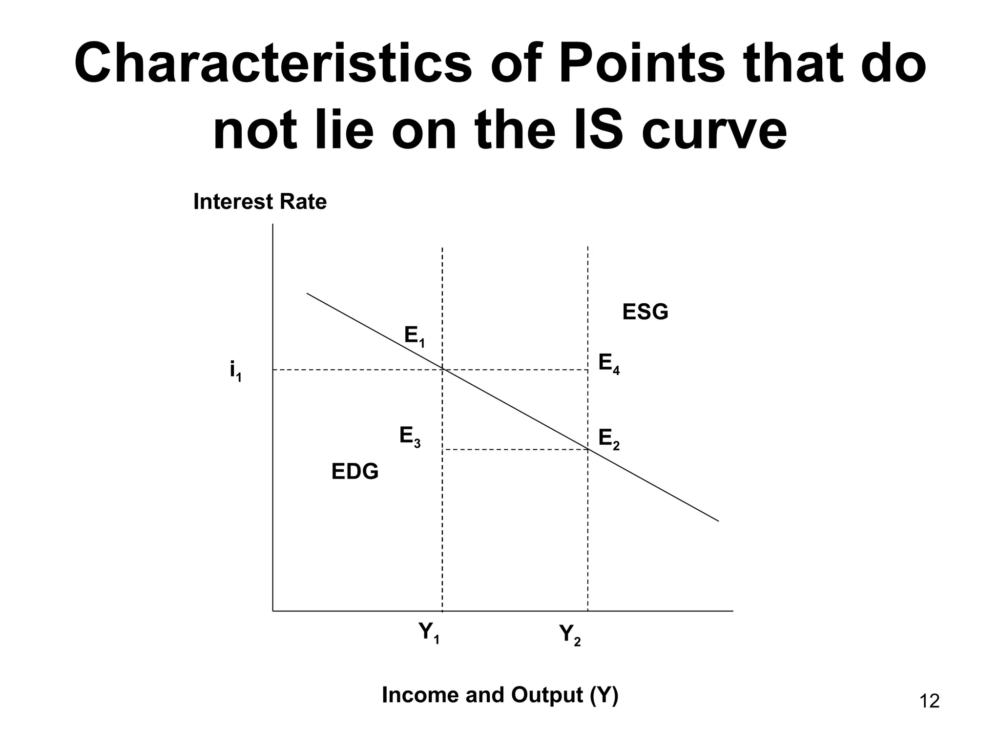
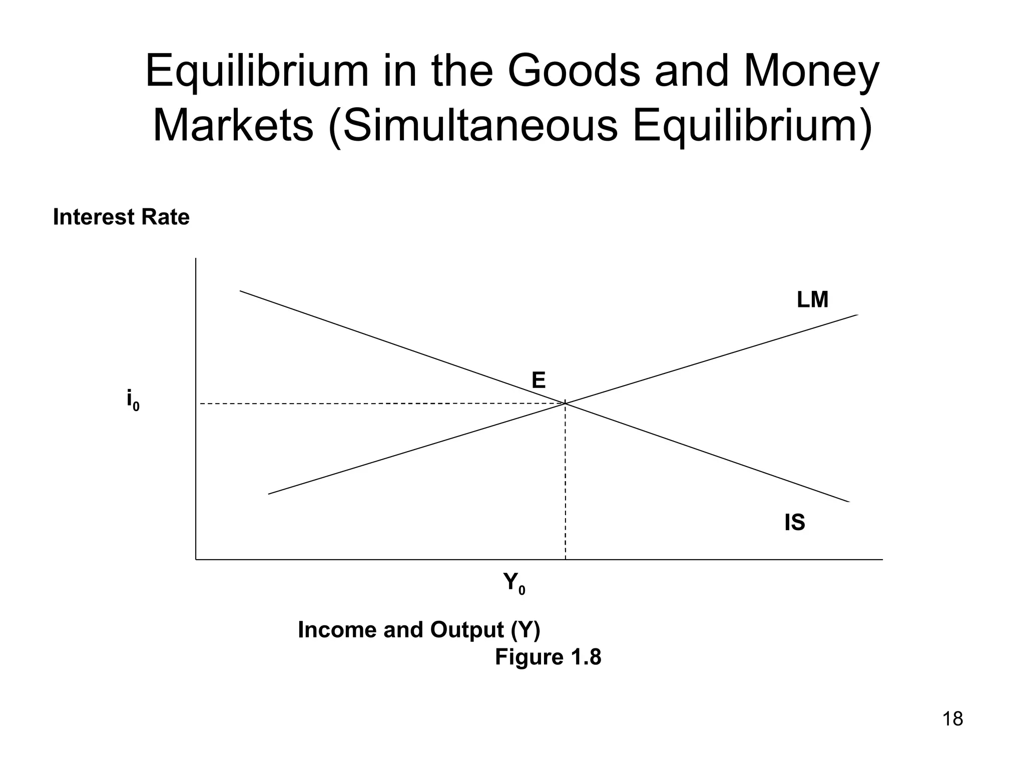
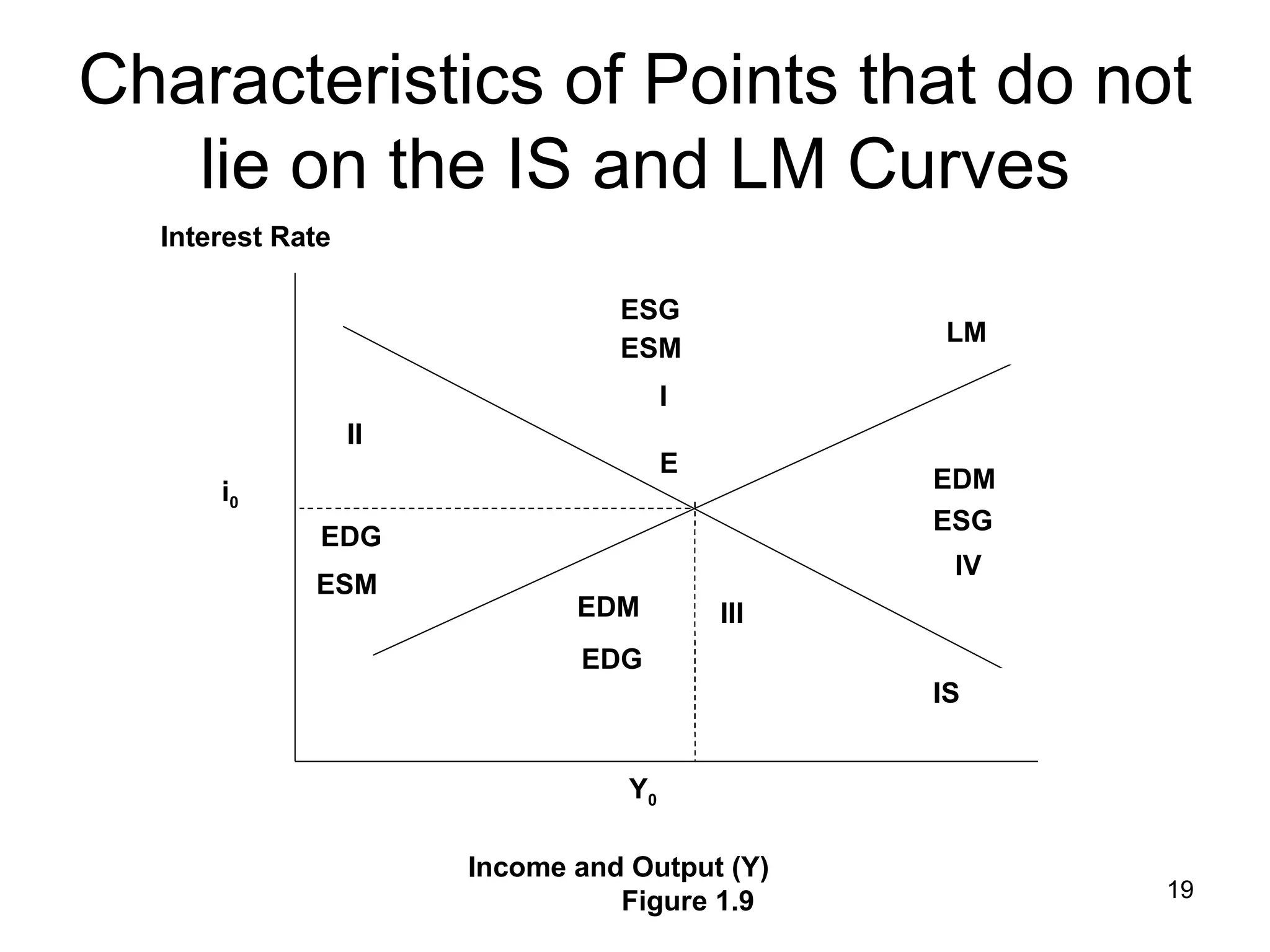
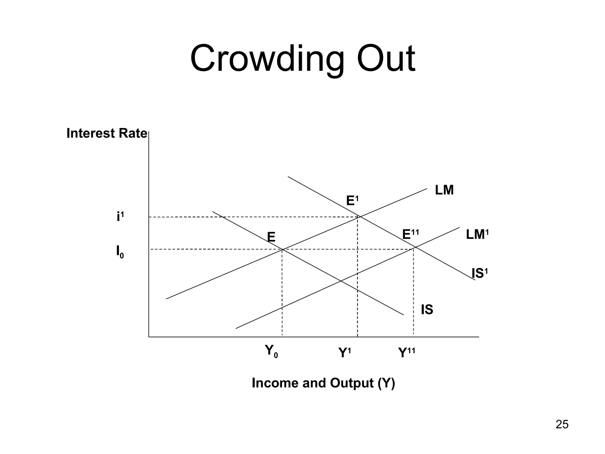
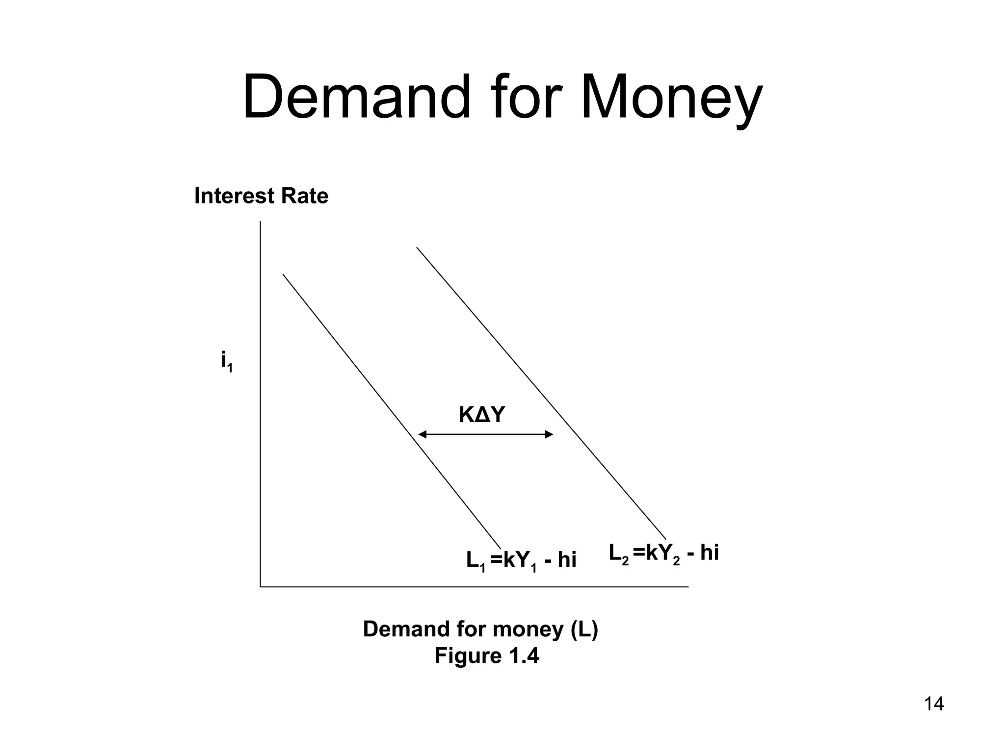
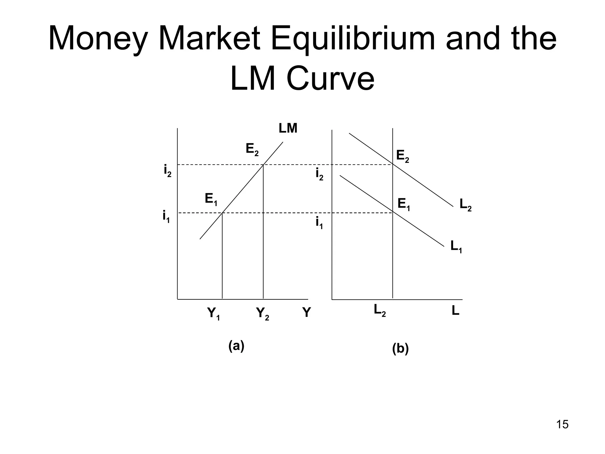
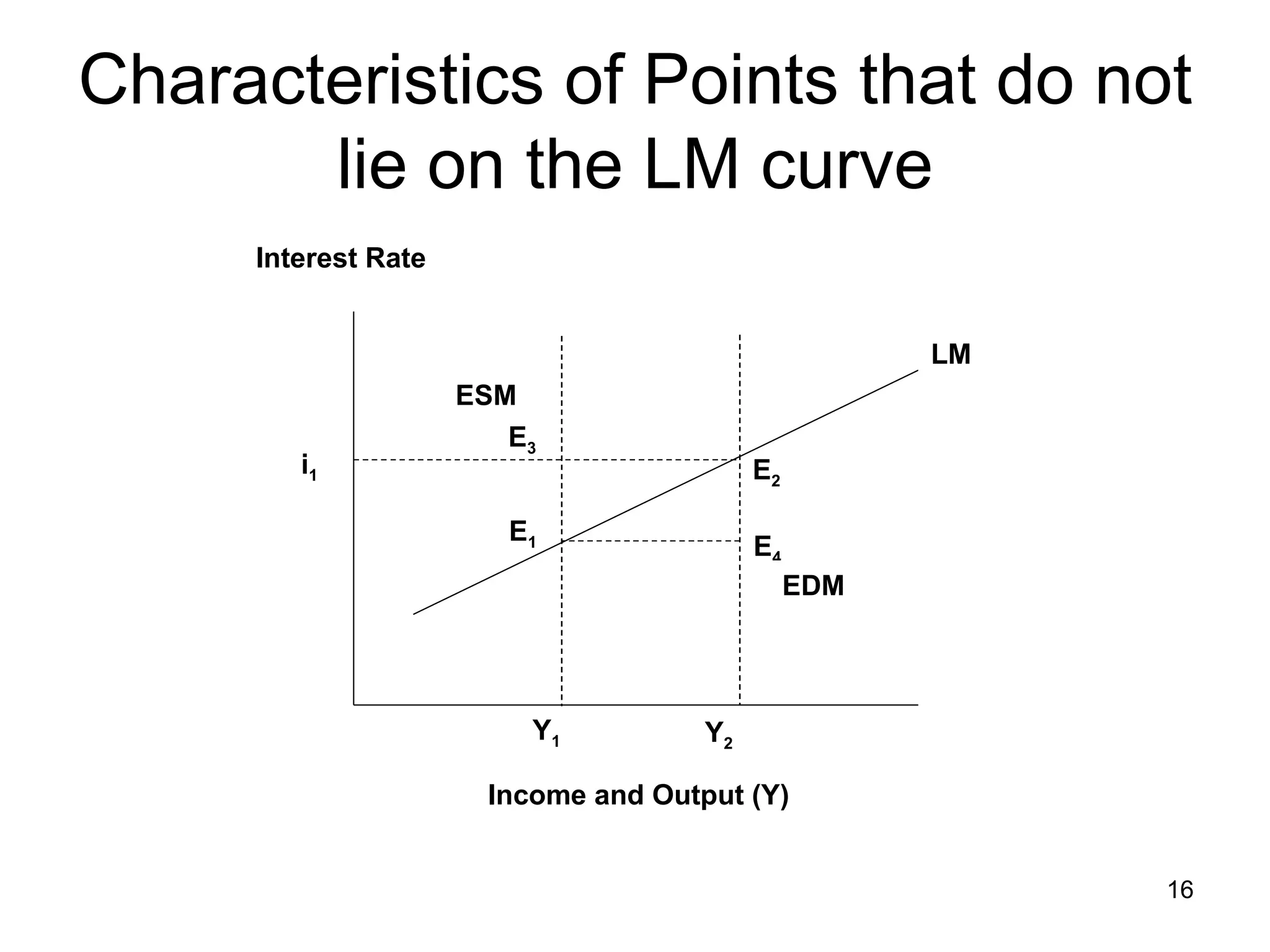
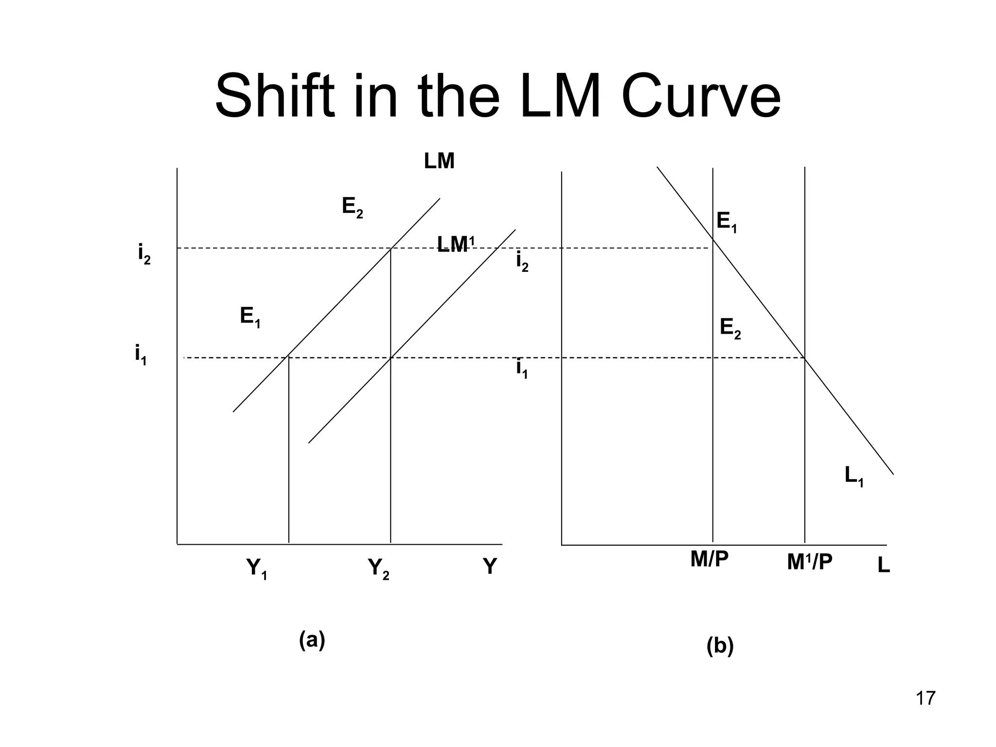
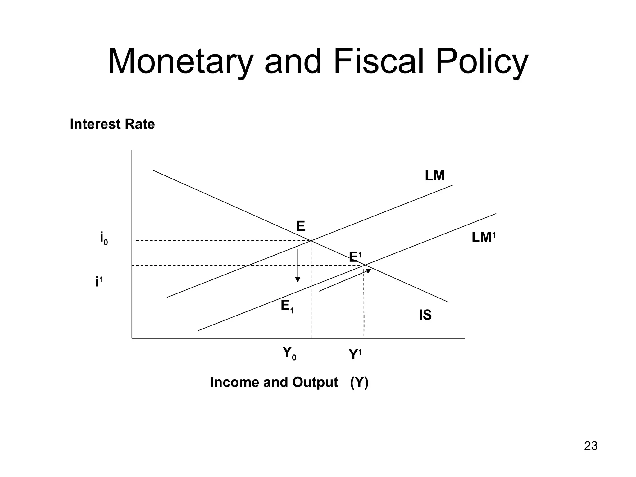
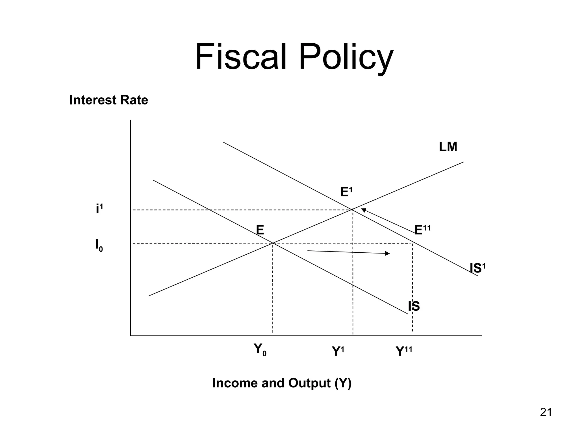
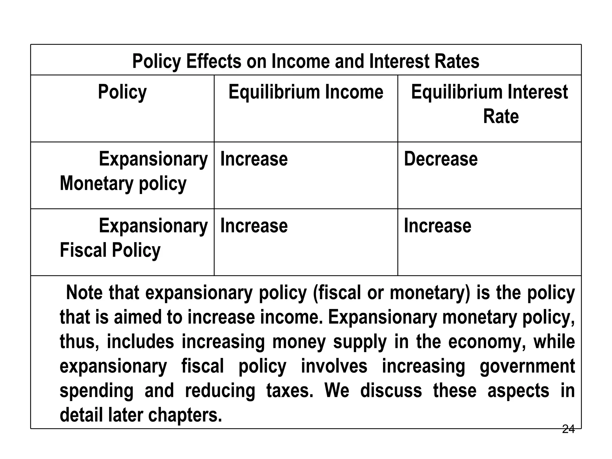
The document outlines key concepts related to the goods market, IS curve, money market, and LM curve. It discusses how: - The IS curve shows combinations of interest rates and income where saving equals investment in the goods market. - The LM curve shows combinations of interest rates and income where demand for money equals supply of money in the money market. - Equilibrium in both markets simultaneously determines the equilibrium interest rate and income on the IS-LM model. Fiscal and monetary policies can shift the curves and impact equilibrium.

1. Income Determination Model Including Money and Interest

2. Session Outline The Goods Market and the IS Curve Deriving the IS Curve The Money Market and the LM Curve Deriving the LM Curve

3. The Goods Market and IS Curve ‘ IS CURVE’ “ IS curve shows different combinations of interest rates and income levels at which saving (S) is equal to investment (I)”

4. The Goods Market and the IS Curve "Good market is in equilibrium when saving equals investment." The goods market equilibrium curve, the IS curve shows different combinations of interest rates and income levels at which saving (S) is equal to investment (I).

5. Investment Function Generally, businesses borrow to purchase investment goods. Higher the interest rates , lower the profitability of the investment. Hence, firms want to borrow and invest more when interest rates are lower; this implies an inverse relationship between rate of interest and investment. Here the investment is 'planned' investment spending because only planned investment depends on the interest rate.

6. Investment Function Investment Function = Where, Ї is the autonomous investment (that is, independent of both income and interest rate), ‘i' is the rate of interest and coefficient ‘ θ ’ measures the responsiveness of investment to changes in interest rate Planned investment spending Interest rate

7. The slope of the investment schedule shows the sensitiveness (responsiveness) of planned investment spending with respect of interest rate. If investment is highly responsive to interest rate, a small change in interest rate leads to a greater change in investment.

8. A flatter investment schedule shows higher responsiveness. If the investment responds very little to the interest rates, then the schedule would be nearly vertical. As the investment curve shows the relationship between interest rate and planned investment spending, a change in the investment due to change in the factors other than interest rate would lead to a shift in the investment schedule. Thus, if autonomous investment changes the schedule shifts right or left.

9. Both saving and investment are affected by interest rate fluctuations. While saving is directly related to interest rate, investments are inversely related to rate of interest. In other words, people save more/less when interest rates are high/low. Conversely, they invest less/more when interest rates are high/less.

10. Deriving the IS Curve 45 0 A – i 1 A – i 2 (AD 1 ) i 1 i 2 E 2 E 1 E 1 E 2 Y 1 Y 2 Income, output (a) Y 1 Y 2 Income, output (b) Interest rate Aggregate demand IS (AD 2 )

11. Derivation of IS curve At a given interest rate, equilibrium in panel (a) determines the income level. A drop in the interest rate increases aggregate demand. The IS curve shown in panel (b) depicts the resulting inverse relationship between interest rates and income.

12. Characteristics of Points that do not lie on the IS curve i 1 Interest Rate Y 2 Y 1 E 3 E 2 E 4 E 1 ESG EDG Income and Output (Y)

13. The Money Market and the LM Curve ‘ LM’ CURVE "LM curve shows different combinations of interest rates and income (or output) at which demand for money (L) equals supply of money (M)"

14. Demand for Money L 1 =kY 1 - hi i 1 Interest Rate KΔY L 2 =kY 2 - hi Demand for money (L) Figure 1.4

15. Money Market Equilibrium and the LM Curve i 2 i 1 LM L i 1 i 2 L 2 E 1 E 2 E 2 E 1 Y 2 Y 1 L 2 L 1 Y (a) (b)

16. Characteristics of Points that do not lie on the LM curve ESM i 1 Interest Rate Y 2 Y 1 E 1 E 4 E 2 E 3 EDM Income and Output (Y) LM

17. Shift in the LM Curve M 1 /P LM 1 L 1 i 2 i 1 LM L i 1 i 2 M/P E 2 E 1 E 2 E 1 Y 2 Y 1 Y (a) (b)

18. Equilibrium in the Goods and Money Markets (Simultaneous Equilibrium) i 0 Interest Rate Y 0 E Income and Output (Y) Figure 1.8 LM IS

19. Characteristics of Points that do not lie on the IS and LM Curves III II ESM i 0 ESG ESM Interest Rate Y 0 E EDM Income and Output (Y) Figure 1.9 LM EDM EDG ESG EDG I IV IS

20. Region Goods Market Money Market Disequilibrium Output Disequilibrium Interest Rate I ESG Falls ESM Falls II EDG Rises ESM Falls III EDG Rises EDM Rises IV ESG Falls EDM Rises

21. Fiscal Policy I 0 IS 1 E E 11 i 1 Interest Rate Y 0 E 1 Income and Output (Y) LM IS Y 1 Y 11

22. The Transmission Mechanism The Transmission Mechanism Step One Step Two Change in aggregate demand results in adjustments in output and income. Change in real money supply Adjustments in the portfolio, leading to a change in asset prices and interest rates Changes in interest rates lead to change in aggregate demand

23. Monetary and Fiscal Policy LM 1 E 1 E 1 i 1 i 0 Interest Rate Y 0 E Income and Output (Y) LM IS Y 1

24. Policy Effects on Income and Interest Rates Policy Equilibrium Income Equilibrium Interest Rate Expansionary Monetary policy Increase Decrease Expansionary Fiscal Policy Increase Increase Note that expansionary policy (fiscal or monetary) is the policy that is aimed to increase income. Expansionary monetary policy, thus, includes increasing money supply in the economy, while expansionary fiscal policy involves increasing government spending and reducing taxes. We discuss these aspects in detail later chapters.

25. Crowding Out I 0 IS 1 E E 11 i 1 Interest Rate Y 0 E 1 Income and Output (Y) LM IS Y 1 Y 11 LM 1