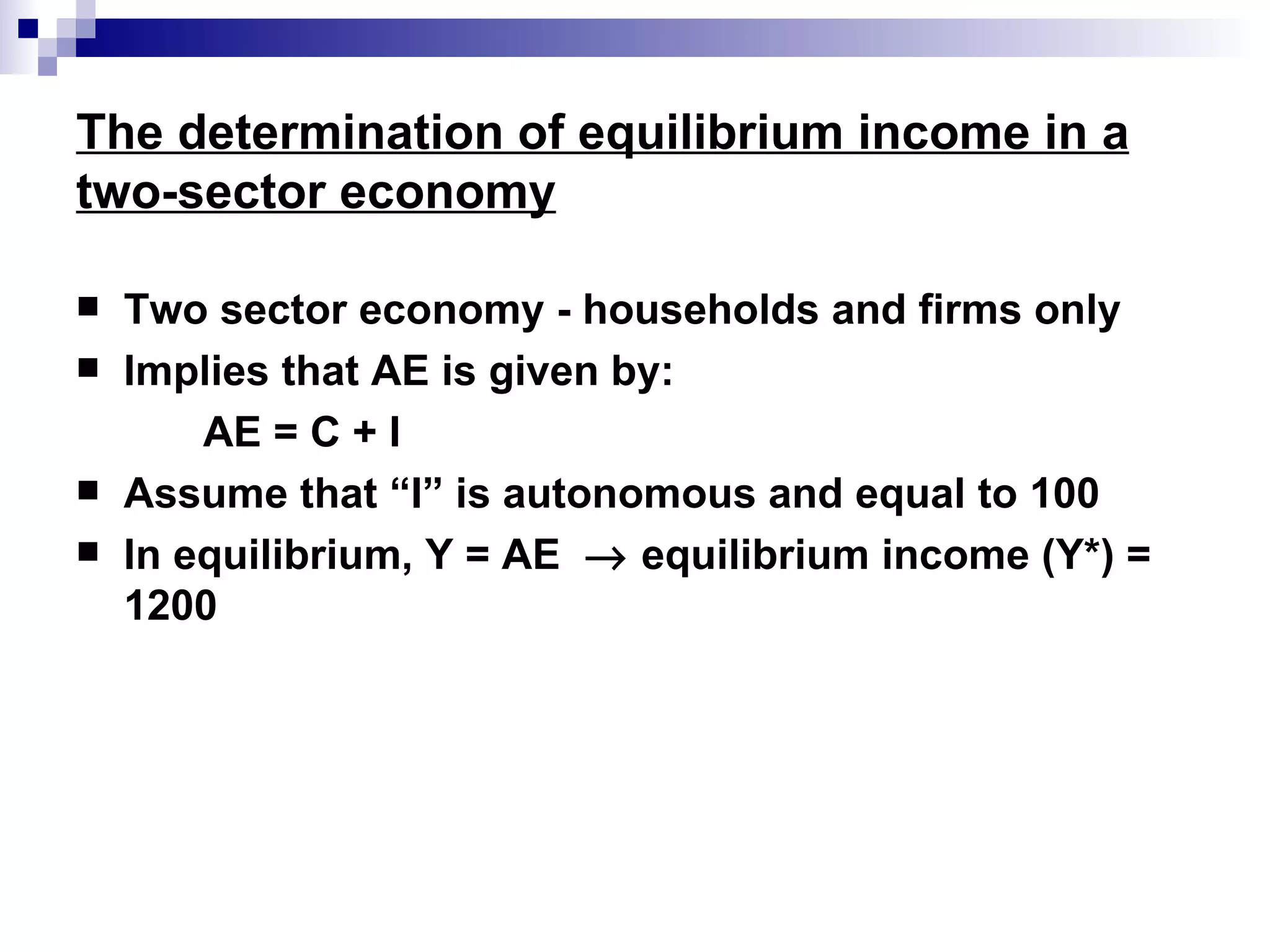
This chapter discusses how to determine national income and its fluctuations. It introduces the concepts of aggregate expenditure (AE), equilibrium income, the consumption function, savings function, investment, and the multiplier. AE is the total planned spending in the economy. Equilibrium occurs when AE equals national income (Y). The chapter shows that an increase in investment (I) or autonomous consumption will increase AE and equilibrium Y through the multiplier effect. It also discusses the "paradox of thrift" where an increase in savings can reduce income.

1. Chapter 9: THE DETERMINATION OF NATIONAL INCOME Economics 11-UPLB Prepared by TBParis 09/12/07

2. Main Objective of the Chapter To explain fluctuations in national income. helps government, researchers, and businessmen formulate targets, policies, and business decisions. gives them an in­sight into the effects of their decisions. need to explain how it is determined. identify the factors that cause national income to change.

3. Chapter Organization Section 9.1 - framework for analyzing changes in national income. Section 9.2 - how changes in income affect consumption spending. Section 9.3, introduces the role of the multiplier effects following a change in aggregate expenditure. Section 9.4 presents an algebraic treatment of the concepts developed

4. Aggregate Expenditure and Equilibrium Income Definition of aggregate expenditure and equilibrium income How the economy adjusts to its equilibrium position. How changes in aggregate expenditure affect equilibrium income.

5. Aggregate Expenditure and Equilibrium National Output Aggregate expenditure (AE) total amount that all economic agents want or plan to spend on domestic goods and services. the planned spending of households, firms, government, and foreigners.

6. Aggregate Expenditure AE = C + I + G + (X-M) consumption (C), investment (I), government spending (G), and exports less imports (X-M). Note that AE is not the same as GDP. AE represents planned spending GDP represents actual spending or output.

7. Aggregate Expenditure (AE) and National Output (Y) AE and Y are not necessarily equal: Firms formulate their production plans with an estimate of the quantities that people want to buy. A mistake on their part will cause production to exceed or fall below the amounts that people want to buy.

8. What if AE and Y are not equal? If AE < Y people want to buy less than what has been produced so firms will accumulate inventories. firms will reduce production If AE >Y What people want to buy is greater than actual production so inventories will decline. firms will increase production

9. Equilibrium National Income AE = Y Can be depicted by the intersection between the AE schedule and the 45 degree line

10. The 45 0 line The 45-degree line is a tool that assists us in identifying the economy's equilibrium position. Property: every point along this line depicts a situation wherein the value of the variable on the horizontal axis (in this case actual output, (Y) is equal to its counterpart on the vertical axis (AE).

11. 0 100 100 45 0 line 45 0 200 200

12. 45º E 0 AE 20 AE 0 20 Output, income (in pesos) Aggregate expenditure (in pesos) Y Y*

13. Equilibrium Income (Y*) When AE is equal to Y there is no reason for firms to adjust production. this suggests that the economy is in equilibrium. Equilibrium requires the equality between income and aggregate expenditure. That is, Y = AE.

14. Changes in AE and Income Suppose that the economy's aggregate expenditure schedule shifts upward AE 0 to AE 1 , E quilibrium point will move from E 0 to E 1 . As a result, the economy experiences an increase in equilibrium income from Y O * to Y 1 *

15. 45° AE 0 E 0 E 1 AE 1 20 30 AE 0 20 30 Y Output, income (in pesos) Aggregate expenditure (in pesos) Y 0 Y 1

16. Consumption and Income Keynes (1936) suggested that consumption spending (C) tends to increase with income. In other words, households with higher incomes tend to spend more. There is a positive relationship between consumption spending and income

17. 0.75 150 200 1,400 1,600 0.75 150 200 1,250 1,400 0.75 150 200 1,100 1,200 0.75 150 200 950 1,000 0.75 150 200 800 800 0.75 150 200 650 600 0.75 150 200 500 400 0.75 150 200 350 200 _ — — 200 0 (∆C/∆Y) (∆C) (∆Y) (C) (Y) mpc Change in consumption Change In income Consumption Income (5) (4) (3) (2) (1) TABLE 9.1. Consumption and income (in pesos).

18. Consumption and income Higher levels of income correspond to higher levels of consumption spending When income is equal to zero, consumption spending is equal to 200. Consumption spending and income are equal at each other when income = 800. When income is less than 800, consumption is higher than income. When income is greater than 800, consumption less than income

19. 0 45 0 200 Consumption Spending (in pesos) Output, Income (in pesos) 400 600 800 1000 800 1200 1600 400 1200 1400 1600 C Y THE CONSUMPTION SCHEDULE Y

20. Consumption and Income Observations from values above: (a) autonomous consumption spending - component of consumption spending that does not depend on income - equal to 200 in example (b) marginal propensity to consume (mpc) - shows the increase in consumption spending for a one peso increase in income;

21. Marginal Propensity to Consume MPC or the marginal propensity to consume represents the change in consumption spending that arises from a one peso change in income. Value of MPC is between 0 and 1. MPC=0.75 means that a one peso increase in income leads to a 75-centavo increase in consumption spending.

22. Marginal propensity to consume In example above, ∆ C = 150 for ∆Y = 200. Hence,

23. Consumption Function Consumption Function : C = c + mpc.Y C = 200 + 0.75Y

24. Savings and Income Sum of consumption spending and savings (S) must equal income. In symbols, Y = C + S. Subtracting C from both sides of this equation leads to S = Y - C.

25. Relationship bet. Income and Savings 0.25 50 150 200 200 1400 1600 0.25 50 150 200 150 1200 1400 0.25 50 150 200 100 1000 1200 0.25 50 150 200 50 950 1000 0.25 50 150 200 0 800 800 0.25 50 150 200 -50 650 600 0.25 50 150 200 -100 500 400 0.25 50 150 200 -150 350 200 - - - - -200 200 0 ∆ S ∆ Y ∆ S ∆ C ∆ Y S C Y MPS (6) (5) (4) (3) (2) (1)

26. Savings and income Savings - that component of income that is not allocated to consumption. S = Y – C How is savings linked to income?  Y   S.

27. Savings and Income Marginal propensity to save (MPS) is the increase in savings for a one peso increase in income; In the example above, ∆S = 50 for ∆ Y = 200. Implies that

28. Savings function Note: MPC+MPS = 1 Savings schedule – listing of values of savings at each levels of income Savings function – in equation form S = -200 + .25Y

29. Relationship between mpc and mpc

30. S -200 -50 150 0 400 800 1,200 1,600 Income (in pesos) Savings (in pesos) Y S F9.4 Propensity to Save

31. The determination of equilibrium income in a two-sector economy Two sector economy - households and firms only Implies that AE is given by: AE = C + I Assume that “I” is autonomous and equal to 100 In equilibrium, Y = AE  equilibrium income (Y*) = 1200

32. Table 9.3 Consumption, Investment and Equilibrium Income. 1,350 100 150 1,250 1,400 1,200 100 100 1,100 1,200 1,050 100 50 950 1,000 900 100 0 800 800 750 100 -50 650 600 600 100 -100 500 400 AE I S C Y

33. E 0 S I -200 100 0 800 1,200 1,600 Income (in pesos) Y Y* (B) S, I (A) E 0   Fig 9.5 C+I = AE C 0 400 800 1,200 1,600 Y 45º AE 300 200  Y* 

34. Investment and Multiplier Suppose that investment I increases from 100M pesos to 200M pesos What happens to equilibrium income? Equilibrium income Y* will increase Not by 100M But by a multiplied amount!! WHY???

35. Table 9.4 Effects of a 100 peso increase in investment. 1750 200 250 1550 1800 1600 200 200 1400 1600 1450 200 150 1,250 1,400 1300 200 100 1,100 1,200 1150 200 50 950 1,000 1000 200 0 800 800 850 200 -50 650 600 700 200 -100 500 400 AE I S C Y

36. Aggregate Expenditure (in pesos) AE 0 AE 1 Y 0 Y* 0 Y* 1 A B E 1 E 0 1200 1600 ∆ I=100 The effect of an increase in investment AE Y 45 o 300 400 ∆ Y=400

37. Calculation of equilibrium income In numerical example,

38. For I = 200, Y* = 1,600 Hence, if I  from 100 to 200  Y*  from 1200 to 1600. In other words,  

39. The concept of the multiplier Increase in Y is greater than increase in I. Why? Multiplier (  ) - measures the change in equilibrium income as a result of a one-peso change in the sum of the autonomous components of AE;

40. The multiplier concept … … … … mpc n-1 •100 0 mpc•[ mpc n-2 •100] n mpc 2 •100 0 mpc• [mpc•100] 3 mpc•100 0 mpc•[100] 2 100 100 0 1 ∆ Y ∆ I = ∆ C + Round

41. Calculation of the multiplier:

42. Calculation of multiplier With the mpc = 0.75, The multiplier is used determine the amount by which Y* changes in response to a change in investment.

43. So the total change in income is given by:  Y =  I + mpc  I + mpc 2  I +mpc 3  I +… = (1 + mpc + mpc 2 + mpc 3 …) .  I or

44. The Multiplier

45. The Paradox of Thrift Many people believe that higher savings lead to higher income. In the present model, we get a result that is contrary to this belief. In other words, equilibrium income falls when people want to save more. Idea: the attempt to achieve higher savings may reduce equilibrium income

46. S 0 Income (in pesos) Savings (in pesos) Y S,I S 1 I Y 0 Y 1 Fig 9.7 0 The Paradox of Thrift

47. End Chapter 9: