Downloaded 52 times

![Government’s Role
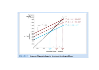
Government spending and taxes
can be used to change the position of the
aggregate demand function
Government spending adds directly
to aggregate demand
Taxes do not affect aggregate demand directly
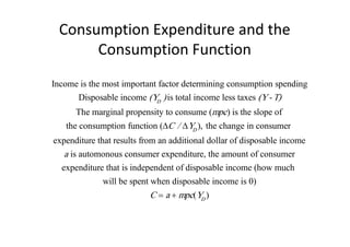
C = a + [ mpc × (Y − T )] = a + ( mpc × Y) − ( mpc × T )
If taxes change, consumer expenditure changes
in the opposite direction
∆C = - mpc × ∆T](https://image.slidesharecdn.com/5islm1-120502144309-phpapp01/85/5-islm-1-12-320.jpg)
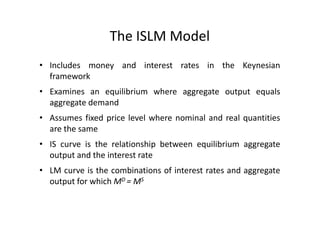
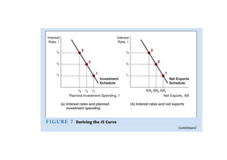
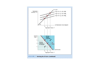
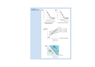
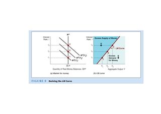
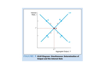


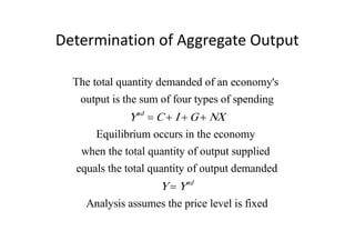
The document summarizes the IS-LM model, which examines macroeconomic equilibrium where aggregate output equals aggregate demand. It discusses: 1) The IS curve, which shows the relationship between equilibrium output and interest rates based on investment spending and net exports. 2) The LM curve, which connects points where money demand equals money supply, showing the interest rate needed for equilibrium at each output level. 3) How the intersection of the IS and LM curves determines equilibrium in both the goods market and money market simultaneously, with output and interest rate satisfying both markets.


