This section discusses three-dimensional stress and strain. It introduces the traction vector and its components, which are represented by the stress tensor. Cauchy's law relates the traction vector on a surface to the stress tensor and the surface normal. The stress tensor transforms between coordinate systems according to the tensor transformation rule. Stresses can be resolved into normal and shear components on any plane through a point.

1. Section 7.2
Solid Mechanics Part II Kelly201
7.2 Analysis of Three Dimensional Stress and Strain
The concept of traction and stress was introduced and discussed in Part I, §3.1-3.5. For
the most part, the discussion was confined to two-dimensional states of stress. Here, the
fully three dimensional stress state is examined. There will be some repetition of the
earlier analyses.
7.2.1 The Traction Vector and Stress Components
Consider a traction vector t acting on a surface element, Fig. 7.2.1. Introduce a Cartesian
coordinate system with base vectors ie so that one of the base vectors is a normal to the
surface and the origin of the coordinate system is positioned at the point at which the
traction acts. For example, in Fig. 7.1.1, the 3e direction is taken to be normal to the
plane, and a superscript on t denotes this normal:
332211
)( 3
eeet e
ttt ++= (7.2.1)
Each of these components it is represented by ijσ where the first subscript denotes the
direction of the normal and the second denotes the direction of the component to the
plane. Thus the three components of the traction vector shown in Fig. 7.2.1 are
333231 ,, σσσ :
333232131
)( 3
eeet e
σσσ ++= (7.2.2)
The first two stresses, the components acting tangential to the surface, are shear stresses
whereas 33σ , acting normal to the plane, is a normal stress.
Figure 7.2.1: components of the traction vector
Consider the three traction vectors )()()( 321
,, eee
ttt acting on the surface elements whose
outward normals are aligned with the three base vectors je , Fig. 7.2.2a. The three (or six)
surfaces can be amalgamated into one diagram as in Fig. 7.2.2b.
In terms of stresses, the traction vectors are
)( 3e
t
2x
1x
3x
)ˆ(n
t
1e 2e
3e
32σ 31σ
33σ

2. Section 7.2
Solid Mechanics Part II Kelly202
( )
( )
( )
33323231
32322221
31321211
3
2
eeet
eeet
eeet
1
e
1
e
1
e1
σσσ
σσσ
σσσ
++=
++=
++=
or ( )
jij
i
et e
σ= (7.2.3)
Figure 7.2.2: the three traction vectors acting at a point; (a) on mutually orthogonal
planes, (b) the traction vectors illustrated on a box element
The components of the three traction vectors, i.e. the stress components, can now be
displayed on a box element as in Fig. 7.2.3. Note that the stress components will vary
slightly over the surfaces of an elemental box of finite size. However, it is assumed that
the element in Fig. 7.2.3 is small enough that the stresses can be treated as constant, so
that they are the stresses acting at the origin.
Figure 7.2.3: the nine stress components with respect to a Cartesian coordinate
system
The nine stresses can be conveniently displayed in 33× matrix form:
21σ11σ
31σ
12σ
22σ
32σ
23σ
33σ
13σ
3x
2x
1x
1e
( )1e
t
01 =x 02 =x 03 =x
2e 3e
( )3e
t
( )2e
t
1x
2x
3x
1x
2x
3x
1x
2x
3x
3x
2x
2e
3e
1e
( )1e
t
( )2e
t
( )3e
t
1x
)a(
)b(

3. Section 7.2
Solid Mechanics Part II Kelly203
[ ]
⎥
⎥
⎦
⎤
⎢
⎢
⎣
⎡
=
333231
232221
131211
σσσ
σσσ
σσσ
σij (7.2.4)
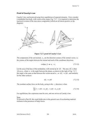
It is important to realise that, if one were to take an element at some different orientation
to the element in Fig. 7.2.3, but at the same material particle, for example aligned with
the axes 321 ,, xxx ′′′ shown in Fig. 7.2.4, one would then have different tractions acting and
the nine stresses would be different also. The stresses acting in this new orientation can
be represented by a new matrix:
[ ]
⎥
⎥
⎦
⎤
⎢
⎢
⎣
⎡
′′′
′′′
′′′
=′
333231
232221
131211
σσσ
σσσ
σσσ
σij (7.2.5)
Figure 7.2.4: the stress components with respect to a Cartesian coordinate system
different to that in Fig. 7.2.3
7.2.2 Cauchy’s Law
Cauchy’s Law, which will be proved below, states that the normal to a surface, iin en = ,
is related to the traction vector iit et n
=)(
acting on that surface, according to
jjii nt σ= (7.2.6)
Writing the traction and normal in vector form and the stress in 33× matrix form,
[ ] [ ] [ ]
⎥
⎥
⎦
⎤
⎢
⎢
⎣
⎡
=
⎥
⎥
⎦
⎤
⎢
⎢
⎣
⎡
=
⎥
⎥
⎥
⎦
⎤
⎢
⎢
⎢
⎣
⎡
=
3
2
1
333231
232221
131211
)(
3
)(
2
)(
1
)(
,,
n
n
n
n
t
t
t
t iiji
σσσ
σσσ
σσσ
σ
n
n
n
n
(7.2.7)
and Cauchy’s law in matrix notation reads
1x′
2x′
3x′
11σ′
12σ′
13σ′31σ′
33σ′
32σ′
22σ′
21σ′
23σ′

4. Section 7.2
Solid Mechanics Part II Kelly204
⎥
⎥
⎦
⎤
⎢
⎢
⎣
⎡
⎥
⎥
⎦
⎤
⎢
⎢
⎣
⎡
=
⎥
⎥
⎥
⎦
⎤
⎢
⎢
⎢
⎣
⎡
3
2
1
332313
322212
312111
)(
3
)(
2
)(
1
n
n
n
t
t
t
σσσ
σσσ
σσσ
n
n
n
(7.2.8)
Note that it is the transpose stress matrix which is used in Cauchy’s law. Since the stress
matrix is symmetric, one can express Cauchy’s law in the form
jiji nt σ= Cauchy’s Law (7.2.9)
Cauchy’s law is illustrated in Fig. 7.2.5; in this figure, positive stresses ijσ are shown.
Figure 7.2.5: Cauchy’s Law; given the stresses and the normal to a plane, the
traction vector acting on the plane can be determined
Normal and Shear Stress
It is useful to be able to evaluate the normal stress Nσ and shear stress Sσ acting on any
plane, Fig. 7.2.6. For this purpose, note that the stress acting normal to a plane is the
projection of )(n
t in the direction of n ,
)(n
tn ⋅=Nσ (7.2.10)
The magnitude of the shear stress acting on the surface can then be obtained from
22)(
NS σσ −= n
t (7.2.11)
3x
2x
1x
n
( )n
t
23σ
13σ
33σ
12σ
22σ
32σ
31σ
21σ
11σ
( )n
3t
( )n
1t
( )n
2t

5. Section 7.2
Solid Mechanics Part II Kelly205
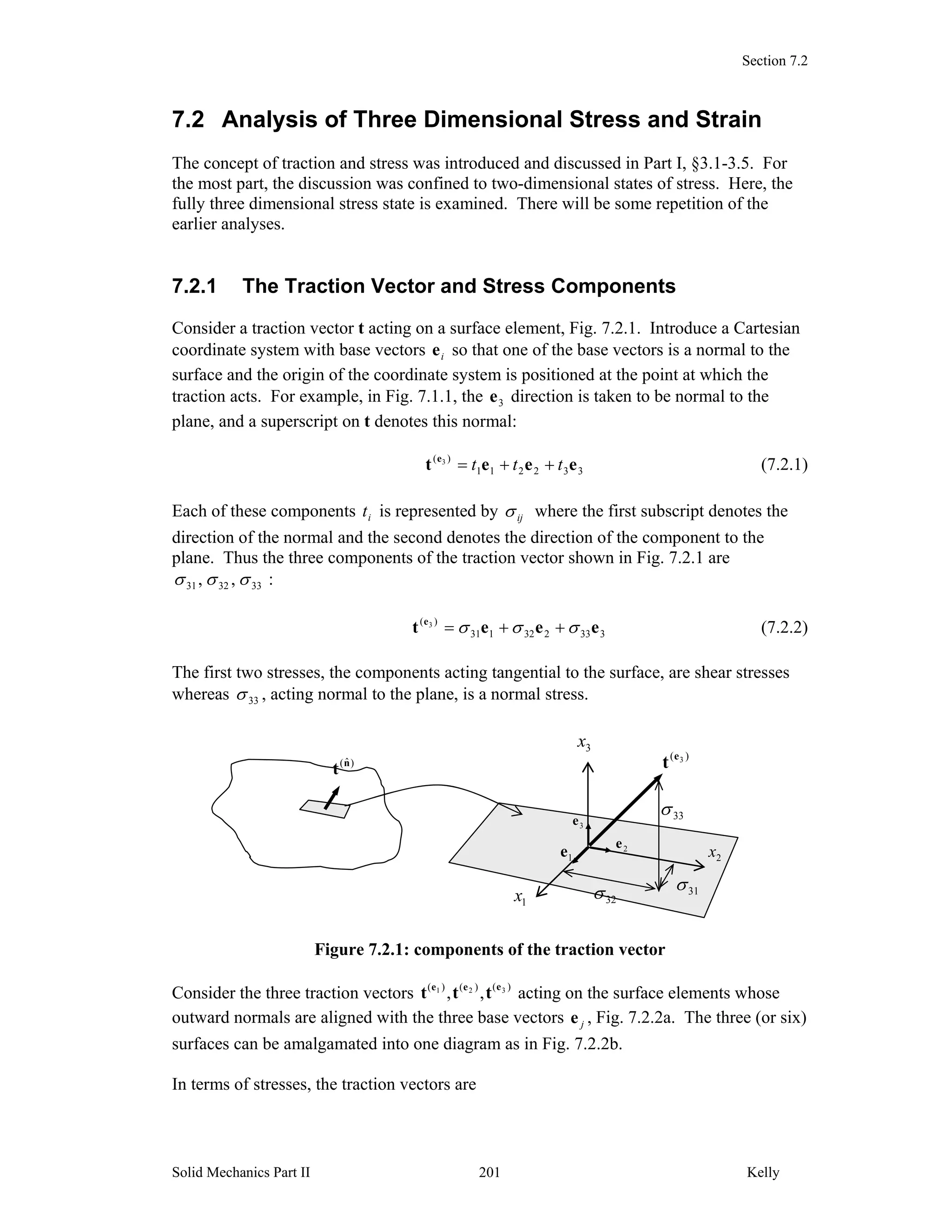
Figure 7.2.6: the normal and shear stress acting on an arbitrary plane through a
point
Example
The state of stress at a point with respect to a Cartesian coordinates system 3210 xxx is
given by:
[ ]
⎥
⎥
⎥
⎦
⎤
⎢
⎢
⎢
⎣
⎡
−
−=
123
221
312
ijσ
Determine:
(a) the traction vector acting on a plane through the point whose unit normal is
321 )3/2()3/2()3/1( eeen −+=
(b) the component of this traction acting perpendicular to the plane
(c) the shear component of traction on the plane
Solution
(a) From Cauchy’s law,
⎥
⎥
⎦
⎤
⎢
⎢
⎣
⎡
−
−
=
⎥
⎥
⎦
⎤
⎢
⎢
⎣
⎡
−⎥
⎥
⎦
⎤
⎢
⎢
⎣
⎡
−
−=
⎥
⎥
⎦
⎤
⎢
⎢
⎣
⎡
⎥
⎥
⎦
⎤
⎢
⎢
⎣
⎡
=
⎥
⎥
⎥
⎦
⎤
⎢
⎢
⎢
⎣
⎡
3
9
2
3
1
2
2
1
123
221
312
3
1
3
2
1
332313
322212
312111
)(
3
)(
2
)(
1
n
n
n
t
t
t
σσσ
σσσ
σσσ
n
n
n
so that 321
)(
ˆ3)3/2( eeet n
−+−= .
(b) The component normal to the plane is
.4.29/22)3/2()3/2(3)3/1)(3/2()(
≈=++−=⋅= nt n
Nσ
(c) The shearing component of traction is
( ) ( ) ( )[ ] ( )[ ]{ } 1.213
2/12
9
22222
3
222)(
≈−−++−=−= NS σσ n
t
■
3x
2x
1x
n
( )n
tNσ
Sσ

6. Section 7.2
Solid Mechanics Part II Kelly206
Proof of Cauchy’s Law
Cauchy’s law can be proved using force equilibrium of material elements. First, consider
a tetrahedral free-body, with vertex at the origin, Fig. 7.2.7. It is required to determine the
traction t in terms of the nine stress components (which are all shown positive in the
diagram).
Figure 7.2.7: proof of Cauchy’s Law
The components of the unit normal, in , are the direction cosines of the normal vector, i.e.
the cosines of the angles between the normal and each of the coordinate directions:
( ) iii n=⋅= enen,cos (7.2.12)
Let the area of the base of the tetrahedran, with normal n, be SΔ . The area 1SΔ is then
αcosSΔ , where α is the angle between the planes, as shown to the right of Fig. 7.2.7;
this angle is the same as that between the vectors n and 1e , so SnS Δ=Δ 11 , and similarly
for the other surfaces:
SnS ii Δ=Δ (7.2.13)
The resultant surface force on the body, acting in the ix direction, is then
SnStSStF jjiijjiii Δ−Δ=Δ−Δ=∑ σσ (7.2.14)
For equilibrium, this expression must be zero, and one arrives at Cauchy’s law.
Note:
As proved in Part III, this result holds also in the general case of accelerating material
elements in the presences of body forces.
3x
2x
1x
n
( )n
t
23σ
13σ
33σ
12σ
22σ
32σ
31σ
21σ
11σ 1SΔ
3SΔ
•
•
n
2SΔ
α
1e

7. Section 7.2
Solid Mechanics Part II Kelly207
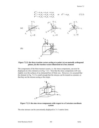
7.2.3 The Stress Tensor
Cauchy’s law 7.2.9 is of the same form as 7.1.24 and so by definition the stress is a
tensor. Denote the stress tensor in symbolic notation by σ . Cauchy’s law in symbolic
form then reads
nσt = (7.2.15)
Further, the transformation rule for stress follows the general tensor transformation rule
7.1.31:
[ ] [ ][ ][ ]
[ ] [ ][ ][ ]QσQσ
QσQσ
T
T
=′=′
′=′=
K
K
pqqjpiij
pqjqipij
QQ
QQ
σσ
σσ
Stress Transformation Rule (7.2.16)
As with the normal and traction vectors, the components and hence matrix representation
of the stress changes with coordinate system, as with the two different matrix
representations 7.2.4 and 7.2.5. However, there is only one stress tensor σ at a point.
Another way of looking at this is to note that an infinite number of planes pass through a
point, and on each of these planes acts a traction vector, and each of these traction vectors
has three (stress) components. All of these traction vectors taken together define the
complete state of stress at a point.
Example
The state of stress at a point with respect to an 3210 xxx coordinate system is given by
[ ]
⎥
⎥
⎦
⎤
⎢
⎢
⎣
⎡
−
−=
120
231
012
ijσ
(a) What are the stress components with respect to axes 3210 xxx ′′′ which are obtained
from the first by a o
45 rotation (positive counterclockwise) about the 2x axis, Fig.
7.2.8?
(b) Use Cauchy’s law to evaluate the normal and shear stress on a plane with normal
( ) ( ) 31 2/12/1 een += and relate your result with that from (a)

8. Section 7.2
Solid Mechanics Part II Kelly208
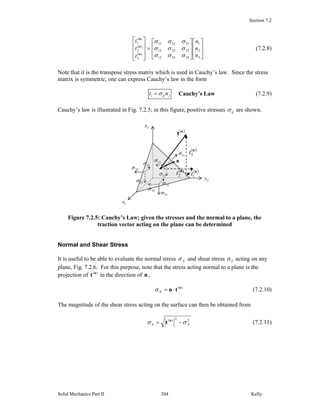
Figure 7.2.8: two different coordinate systems at a point
Solution
(a) The transformation matrix is
[ ]
( ) ( ) ( )
( ) ( ) ( )
( ) ( ) ( ) ⎥
⎥
⎥
⎦
⎤
⎢
⎢
⎢
⎣
⎡
−
=
⎥
⎥
⎥
⎦
⎤
⎢
⎢
⎢
⎣
⎡
′′′
′′′
′′′
=
2
1
2
1
2
1
2
1
332313
322212
312111
0
010
0
,cos,cos,cos
,cos,cos,cos
,cos,cos,cos
xxxxxx
xxxxxx
xxxxxx
Qij
and IQQ =T
as expected. The rotated stress components are therefore
⎥
⎥
⎥
⎦
⎤
⎢
⎢
⎢
⎣
⎡
−
−=
⎥
⎥
⎥
⎦
⎤
⎢
⎢
⎢
⎣
⎡
−⎥
⎥
⎥
⎦
⎤
⎢
⎢
⎢
⎣
⎡
−
−
⎥
⎥
⎥
⎦
⎤
⎢
⎢
⎢
⎣
⎡ −
=
⎥
⎥
⎥
⎦
⎤
⎢
⎢
⎢
⎣
⎡
′′′
′′′
′′′
2
3
2
1
2
1
2
1
2
3
2
1
2
3
2
3
2
1
2
1
2
1
2
1
2
1
2
1
2
1
2
1
333231
232221
131211
3
0
010
0
120
231
012
0
010
0
σσσ
σσσ
σσσ
and the new stress matrix is symmetric as expected.
(b) From Cauchy’s law, the traction vector is
⎥
⎥
⎥
⎦
⎤
⎢
⎢
⎢
⎣
⎡
−=
⎥
⎥
⎥
⎦
⎤
⎢
⎢
⎢
⎣
⎡
⎥
⎥
⎥
⎦
⎤
⎢
⎢
⎢
⎣
⎡
−
−=
⎥
⎥
⎥
⎦
⎤
⎢
⎢
⎢
⎣
⎡
2
1
2
1
2
1
2
1
)(
3
)(
2
)(
1 2
0
120
231
012
n
n
n
t
t
t
so that ( ) ( ) ( ) 321
)(
ˆ2/12/12 eeet n
+−= . The normal and shear stress on the
plane are
2/3)(
=⋅= nt n
Nσ
and
2/3)2/3(3 222)(
=−=−= NS σσ n
t
The normal to the plane is equal to 3e′ and so Nσ should be the same as 33σ ′ and it
is. The stress Sσ should be equal to ( ) ( )2
32
2
31 σσ ′+′ and it is. The results are
1x
1e 22 ee ′=
3e
3e′
22 xx ′=
3x
1e′
1x′
3x′
o
45
o
45

9. Section 7.2
Solid Mechanics Part II Kelly209
displayed in Fig. 7.2.9, in which the traction is represented in different ways, with
components ( ))(
3
)(
2
)(
1 ,, nnn
ttt and ( )333231 ,, σσσ ′′′ .
Figure 7.2.9: traction and stresses acting on a plane
Isotropic State of Stress
Suppose the state of stress in a body is
[ ]
⎥
⎥
⎥
⎦
⎤
⎢
⎢
⎢
⎣
⎡
==
0
0
0
0
00
00
00
σ
σ
σ
δσσ σijij (7.2.17)
One finds that the application of the stress tensor transformation rule yields the very same
components no matter what the new coordinate system{▲Problem 3}. In other words, no
shear stresses act, no matter what the orientation of the plane through the point. This is
termed an isotropic state of stress, or a spherical state of stress. One example of
isotropic stress is the stress arising in a fluid at rest, which cannot support shear stress, in
which case
[ ] [ ]Iσ p−= (7.2.18)
where the scalar p is the fluid hydrostatic pressure. For this reason, an isotropic state of
stress is also referred to as a hydrostatic state of stress.
7.2.4 Principal Stresses
For certain planes through a material particle, there are traction vectors which act normal
to the plane, as in Fig. 7.2.10. In this case the traction can be expressed as a scalar
multiple of the normal vector, nt n
σ=)(
.
3en ′=
22 xx ′=
1x′
2
3
33 =′=σσN
)(n
t
2
3
32 −=′σ
2
1
31 =′σ
2)(
1 =n
t
2
1)(
2 −=n
t
2
1)(
3 =n
t Sσ
1x

10. Section 7.2
Solid Mechanics Part II Kelly210
Figure 7.2.10: a purely normal traction vector
From Cauchy’s law then, for these planes,
⎥
⎥
⎥
⎦
⎤
⎢
⎢
⎢
⎣
⎡
=
⎥
⎥
⎥
⎦
⎤
⎢
⎢
⎢
⎣
⎡
⎥
⎥
⎥
⎦
⎤
⎢
⎢
⎢
⎣
⎡
==
3
2
1
3
2
1
333231
232221
131211
,,
n
n
n
n
n
n
nn ijij σ
σσσ
σσσ
σσσ
σσσ nnσ (7.2.19)
This is a standard eigenvalue problem from Linear Algebra: given a matrix [ ]ijσ , find
the eigenvalues σ and associated eigenvectors n such that Eqn. 7.2.19 holds.
To solve the problem, first re-write the equation in the form
( ) ( )
⎥
⎥
⎥
⎦
⎤
⎢
⎢
⎢
⎣
⎡
=
⎥
⎥
⎥
⎦
⎤
⎢
⎢
⎢
⎣
⎡
⎪
⎭
⎪
⎬
⎫
⎪
⎩
⎪
⎨
⎧
⎥
⎥
⎥
⎦
⎤
⎢
⎢
⎢
⎣
⎡
−
⎥
⎥
⎥
⎦
⎤
⎢
⎢
⎢
⎣
⎡
=−=−
0
0
0
100
010
001
,0,
3
2
1
333231
232221
131211
n
n
n
njijij σ
σσσ
σσσ
σσσ
σδσσ 0nIσ (7.2.20)
or
⎥
⎥
⎦
⎤
⎢
⎢
⎣
⎡
=
⎥
⎥
⎦
⎤
⎢
⎢
⎣
⎡
⎥
⎥
⎦
⎤
⎢
⎢
⎣
⎡
−
−
−
0
0
0
3
2
1
333231
232221
131211
n
n
n
σσσσ
σσσσ
σσσσ
(7.2.21)
This is a set of three homogeneous equations in three unknowns (if one treats σ as
known). From basic linear algebra, this system has a solution (apart from 0=in ) if and
only if the determinant of the coefficient matrix is zero, i.e. if
0det)det(
333231
232221
131211
=
⎥
⎥
⎦
⎤
⎢
⎢
⎣
⎡
−
−
−
=−
σσσσ
σσσσ
σσσσ
σIσ (7.2.22)
Evaluating the determinant, one has the following cubic characteristic equation of the
stress tensor σ ,
032
2
1
3
=−+− III σσσ Characteristic Equation (7.2.23)
and the principal scalar invariants of the stress tensor are
no shear stress – only a normal
component to the traction
n
nt n
σ=)(

11. Section 7.2
Solid Mechanics Part II Kelly211
312312
2
1233
2
3122
2
23113322113
2
31
2
23
2
121133332222112
3322111
2 σσσσσσσσσσσσ
σσσσσσσσσ
σσσ
+−−−=
−−−++=
++=
I
I
I
(7.2.24)
( 3I is the determinant of the stress matrix.) The characteristic equation 7.2.23 can now be
solved for the eigenvalues σ and then Eqn. 7.2.21 can be used to solve for the
eigenvectors n.
Now another theorem of linear algebra states that the eigenvalues of a real (that is, the
components are real), symmetric matrix (such as the stress matrix) are all real and further
that the associated eigenvectors are mutually orthogonal. This means that the three roots
of the characteristic equation are real and that the three associated eigenvectors form a
mutually orthogonal system. This is illustrated in Fig. 7.2.11; the eigenvalues are called
principal stresses and are labelled 321 ,, σσσ and the three corresponding eigenvectors
are called principal directions, the directions in which the principal stresses act. The
planes on which the principal stresses act (to which the principal directions are normal)
are called the principal planes.
Figure 7.2.11: the three principal stresses acting at a point and the three associated
principal directions 1, 2 and 3
Once the principal stresses are found, as mentioned, the principal directions can be found
by solving Eqn. 7.2.21, which can be expressed as
0)(
0)(
0)(
333232131
323222121
313212111
=−++
=+−+
=++−
nnn
nnn
nnn
σσσσ
σσσσ
σσσσ
(7.2.25)
Each principal stress value in this equation gives rise to the three components of the
associated principal direction vector, 321 ,, nnn . The solution also requires that the
magnitude of the normal be specified: for a unit vector, 1=⋅nn . The directions of the
normals are also chosen so that they form a right-handed set.
1
1σ
3σ
2σ
3
2

12. Section 7.2
Solid Mechanics Part II Kelly212
Example
The stress at a point is given with respect to the axes 321 xxOx by the values
[ ]
⎥
⎥
⎦
⎤
⎢
⎢
⎣
⎡
−
−−=
1120
1260
005
ijσ .
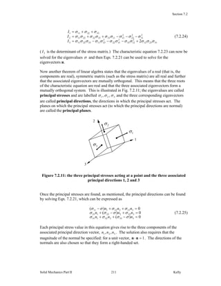
Determine (a) the principal values, (b) the principal directions (and sketch them).
Solution:
(a)
The principal values are the solution to the characteristic equation
0)15)(5)(10(
1120
1260
005
=+−+−=
−−
−−−
−
σσσ
σ
σ
σ
which yields the three principal values 15,5,10 321 −=== σσσ .
(b)
The eigenvectors are now obtained from Eqn. 7.2.25. First, for 101 =σ ,
09120
012160
0005
321
321
321
=−−
=−−
=++−
nnn
nnn
nnn
and using also the equation 12
3
2
2
2
1 =++ nnn leads to 321 )5/4()5/3( een +−= . Similarly,
for 52 =σ and 153 −=σ , one has, respectively,
04120
012110
0000
321
321
321
=−−
=−−
=++
nnn
nnn
nnn
and
016120
01290
00020
321
321
321
=+−
=−+
=++
nnn
nnn
nnn
which yield 12 en = and 323 )5/3()5/4( een += . The principal directions are sketched in
Fig. 7.2.12. Note that the three components of each principal direction, 321 ,, nnn , are the
direction cosines: the cosines of the angles between that principal direction and the three
coordinate axes. For example, for 1σ with 5/4,5/3,0 321 =−== nnn , the angles made
with the coordinate axes 321 ,, xxx are, respectively, 0, 127o
and 37o
.
Figure 7.2.12: principal directions
■
3x
1x
2x
3
ˆn1
ˆn
2
ˆn
o
37

13. Section 7.2
Solid Mechanics Part II Kelly213
Invariants
The principal stresses 321 ,, σσσ are independent of any coordinate system; the 3210 xxx
axes to which the stress matrix in Eqn. 7.2.19 is referred can have any orientation – the
same principal stresses will be found from the eigenvalue analysis. This is expressed by
using the symbolic notation for the problem: nnσ σ= , which is independent of any
coordinate system. Thus the principal stresses are intrinsic properties of the stress state at
a point. It follows that the functions 321 ,, III in the characteristic equation Eqn. 7.2.23
are also independent of any coordinate system, and hence the name principal scalar
invariants (or simply invariants) of the stress.
The stress invariants can also be written neatly in terms of the principal stresses:
3213
1332212
3211
σσσ
σσσσσσ
σσσ
=
++=
++=
I
I
I
(7.2.26)
Also, if one chooses a coordinate system to coincide with the principal directions, Fig.
7.2.12, the stress matrix takes the simple form
[ ]
⎥
⎥
⎦
⎤
⎢
⎢
⎣
⎡
=
3
2
1
00
00
00
σ
σ
σ
σij (7.2.27)
Note that when two of the principal stresses are equal, one of the principal directions will
be unique, but the other two will be arbitrary – one can choose any two principal
directions in the plane perpendicular to the uniquely determined direction, so that the
three form an orthonormal set. This stress state is called axi-symmetric. When all three
principal stresses are equal, one has an isotropic state of stress, and all directions are
principal directions – the stress matrix has the form 7.2.27 no matter what orientation the
planes through the point.
Example
The two stress matrices from the Example of §7.2.3, describing the stress state at a point
with respect to different coordinate systems, are
[ ]
⎥
⎥
⎥
⎦
⎤
⎢
⎢
⎢
⎣
⎡
−
−=
120
231
012
ijσ , [ ]
⎥
⎥
⎥
⎦
⎤
⎢
⎢
⎢
⎣
⎡
−
−=′
2/32/12/1
2/132/3
2/12/32/3
ijσ
The first invariant is the sum of the normal stresses, the diagonal terms, and is the same
for both as expected:
63132 2
3
2
3
1 =++=++=I
The other invariants can also be obtained from either matrix, and are
3,6 32 −== II
■

14. Section 7.2
Solid Mechanics Part II Kelly214
7.2.5 Maximum and Minimum Stress Values
Normal Stresses
The three principal stresses include the maximum and minimum normal stress
components acting at a point. To prove this, first let 321 ,, eee be unit vectors in the
principal directions. Consider next an arbitrary unit normal vector iin en = . From
Cauchy’s law (see Fig. 7.2.13 – the stress matrix in Cauchy’s law is now with respect to
the principal directions 1, 2 and 3), the normal stress acting on the plane with normal n is
( ) ijijNN nnσσσ =⋅=⋅= ,)(
nnσnt n
(7.2.28)
Figure 7.2.13: normal stress acting on a plane defined by the unit normal n
Thus
2
33
2
22
2
11
3
2
1
3
2
1
3
2
1
00
00
00
nnn
n
n
n
n
n
n
N σσσ
σ
σ
σ
σ ++=
⎥
⎥
⎦
⎤
⎢
⎢
⎣
⎡
⎪⎭
⎪
⎬
⎫
⎪⎩
⎪
⎨
⎧
⎥
⎥
⎦
⎤
⎢
⎢
⎣
⎡
⎥
⎥
⎦
⎤
⎢
⎢
⎣
⎡
= (7.2.29)
Since 12
3
2
2
2
1 =++ nnn and, without loss of generality, taking 321 σσσ ≥≥ , one has
( ) Nnnnnnn σσσσσσ =++≥++= 2
33
2
22
2
11
2
3
2
2
2
111 (7.2.30)
Similarly,
( ) 3
2
3
2
2
2
13
2
33
2
22
2
11 σσσσσσ ≥++≥++= nnnnnnN (7.2.31)
Thus the maximum normal stress acting at a point is the maximum principal stress and the
minimum normal stress acting at a point is the minimum principal stress.
3
2
1
n
( )n
tNσ
principal
directions

15. Section 7.2
Solid Mechanics Part II Kelly215
Shear Stresses
Next, it will be shown that the maximum shearing stresses at a point act on planes
oriented at 45o
to the principal planes and that they have magnitude equal to half the
difference between the principal stresses. First, again, let 321 ,, eee be unit vectors in the
principal directions and consider an arbitrary unit normal vector iin en = . The normal
stress is given by Eqn. 7.2.29,
2
33
2
22
2
11 nnnN σσσσ ++= (7.2.32)
Cauchy’s law gives the components of the traction vector as
⎥
⎥
⎦
⎤
⎢
⎢
⎣
⎡
=
⎥
⎥
⎦
⎤
⎢
⎢
⎣
⎡
⎥
⎥
⎦
⎤
⎢
⎢
⎣
⎡
=
⎥
⎥
⎥
⎦
⎤
⎢
⎢
⎢
⎣
⎡
33
22
11
3
2
1
3
2
1
)(
1
)(
1
)(
1
00
00
00
n
n
n
n
n
n
t
t
t
σ
σ
σ
σ
σ
σ
n
n
n
(7.2.33)
and so the shear stress on the plane is, from Eqn. 7.2.11,
( ) ( )22
33
2
22
2
11
2
3
2
3
2
2
2
2
2
1
2
1
2
nnnnnnS σσσσσσσ ++−++= (7.2.34)
Using the condition 12
3
2
2
2
1 =++ nnn to eliminate 3n leads to
( ) ( ) ( ) ( )[ ]2
3
2
232
2
131
2
3
2
2
2
3
2
2
2
1
2
3
2
1
2
σσσσσσσσσσσ +−+−−+−+−= nnnnS (7.2.35)
The stationary points are now obtained by equating the partial derivatives with respect to
the two variables 1n and 2n to zero:
( ) ( ) ( ) ( )[ ]{ }
( ) ( ) ( ) ( )[ ]{ } 02
02
2
232
2
13132322
2
2
2
232
2
13131311
1
2
=−+−−−−=
∂
∂
=−+−−−−=
∂
∂
nnn
n
nnn
n
S
S
σσσσσσσσ
σ
σσσσσσσσ
σ
(7.2.36)
One sees immediately that 021 == nn (so that 13 ±=n ) is a solution; this is the principal
direction 3e and the shear stress is by definition zero on the plane with this normal. In
this calculation, the component 3n was eliminated and 2
Sσ was treated as a function of the
variables ),( 21 nn . Similarly, 1n can be eliminated with ),( 32 nn treated as the variables,
leading to the solution 1en = , and 2n can be eliminated with ),( 31 nn treated as the
variables, leading to the solution 2en = . Thus these solutions lead to the minimum shear
stress value 02
=Sσ .
A second solution to Eqn. 7.2.36 can be seen to be 2/1,0 21 ±== nn (so that
2/13 ±=n ) with corresponding shear stress values ( )2
324
12
σσσ −=S . Two other

16. Section 7.2
Solid Mechanics Part II Kelly216
solutions can be obtained as described earlier, by eliminating 1n and by eliminating 2n .
The full solution is listed below, and these are evidently the maximum (absolute value of
the) shear stresses acting at a point:
21
13
32
2
1
,0,
2
1
,
2
1
2
1
,
2
1
,0,
2
1
2
1
,
2
1
,
2
1
,0
σσσ
σσσ
σσσ
−=⎟
⎠
⎞
⎜
⎝
⎛
±±=
−=⎟
⎠
⎞
⎜
⎝
⎛
±±=
−=⎟
⎠
⎞
⎜
⎝
⎛
±±=
S
S
S
n
n
n
(7.2.37)
Taking 321 σσσ ≥≥ , the maximum shear stress at a point is
( )31max
2
1
σστ −= (7.2.38)
and acts on a plane with normal oriented at 45o
to the 1 and 3 principal directions. This is
illustrated in Fig. 7.2.14.
Figure 7.2.14: maximum shear stress at a point
Example
Consider the stress state examined in the Example of §7.2.4:
[ ]
⎥
⎥
⎦
⎤
⎢
⎢
⎣
⎡
−
−−=
1120
1260
005
ijσ
The principal stresses were found to be 15,5,10 321 −=== σσσ and so the maximum
shear stress is
( )
2
25
2
1
31max =−= σστ
One of the planes upon which they act is shown in Fig. 7.2.15 (see Fig. 7.2.12)
1
3
maxτ
maxτ
principal
directions

17. Section 7.2
Solid Mechanics Part II Kelly217
Figure 7.2.15: maximum shear stress
■
7.2.6 Mohr’s Circles of Stress
The Mohr’s circle for 2D stress states was discussed in Part I, §3.5.4. For the 3D case,
following on from section 7.2.5, one has the conditions
12
3
2
2
2
1
2
3
2
3
2
2
2
2
2
1
2
1
22
2
33
2
22
2
11
=++
++=+
++=
nnn
nnn
nnn
NS
N
σσσσσ
σσσσ
(7.2.39)
Solving these equations gives
( )( )
( )( )
( )( )
( )( )
( )( )
( )( )2313
2
212
3
1232
2
132
2
3121
2
322
1
σσσσ
σσσσσ
σσσσ
σσσσσ
σσσσ
σσσσσ
−−
+−−
=
−−
+−−
=
−−
+−−
=
SNN
SNN
SNN
n
n
n
(7.2.40)
Taking 321 σσσ ≥≥ , and noting that the squares of the normal components must be
positive, one has that
( )( )
( )( )
( )( ) 0
0
0
2
21
2
13
2
32
≥+−−
≤+−−
≥+−−
SNN
SNN
SNN
σσσσσ
σσσσσ
σσσσσ
(7.2.41)
and these can be re-written as
( )[ ] ( )[ ]
( )[ ] ( )[ ]
( )[ ] ( )[ ]2
212
12
212
12
2
312
12
312
12
2
322
12
322
12
σσσσσσ
σσσσσσ
σσσσσσ
−≥+−+
−≤+−+
−≥+−+
NS
NS
NS
(7.2.42)
3x
1x
2x
3
ˆn1
ˆn
2
ˆn
o
37
maxτ

18. Section 7.2
Solid Mechanics Part II Kelly218
If one takes coordinates ( )SN σσ , , the equality signs here represent circles in ( )SN σσ ,
stress space, Fig. 7.2.16. Each point ( )SN σσ , in this stress space represents the stress on
a particular plane through the material particle in question. Admissible ( )SN σσ , pairs are
given by the conditions Eqns. 7.2.42; they must lie inside a circle of centre ( )( )0,312
1
σσ +
and radius ( )312
1
σσ − . This is the large circle in Fig. 7.2.16. The points must lie outside
the circle with centre ( )( )0,322
1
σσ + and radius ( )322
1
σσ − and also outside the circle
with centre ( )( )0,212
1
σσ + and radius ( )212
1
σσ − ; these are the two smaller circles in the
figure. Thus the admissible points in stress space lie in the shaded region of Fig. 7.2.16.
Figure 7.2.16: admissible points in stress space
7.2.7 Three Dimensional Strain
The strain ijε , in symbolic form ε , is a tensor and as such it follows the same rules as for
the stress tensor. In particular, it follows the general tensor transformation rule 7.2.16; it
has principal values ε which satisfy the characteristic equation 7.2.23 and these include
the maximum and minimum normal strain at a point. There are three principal strain
invariants given by 7.2.24 or 7.2.26 and the maximum shear strain occurs on planes
oriented at 45o
to the principal directions.
7.2.8 Problems
1. The state of stress at a point with respect to a 3210 xxx coordinate system is given by
[ ]
⎥
⎥
⎦
⎤
⎢
⎢
⎣
⎡
−−
−=
212
101
212
ijσ
Use Cauchy’s law to determine the traction vector acting on a plane trough this
point whose unit normal is 3/)( 321 eeen ++= . What is the normal stress acting
on the plane? What is the shear stress acting on the plane?
2. The state of stress at a point with respect to a 3210 xxx coordinate system is given by
[ ]
⎥
⎥
⎦
⎤
⎢
⎢
⎣
⎡
−
=
202
013
231
ijσ
Nσ
Sσ
• ••
3σ 2σ 1σ

19. Section 7.2
Solid Mechanics Part II Kelly219
What are the stress components with respect to axes 3210 xxx ′′′ which are obtained
from the first by a o
45 rotation (positive counterclockwise) about the 3x axis
3. Show, in both the index and matrix notation, that the components of an isotropic
stress state remain unchanged under a coordinate transformation.
4. Consider a two-dimensional problem. The stress transformation formulae are then,
in full,
⎥
⎦
⎤
⎢
⎣
⎡ −
⎥
⎦
⎤
⎢
⎣
⎡
⎥
⎦
⎤
⎢
⎣
⎡
−
=⎥
⎦
⎤
⎢
⎣
⎡
′′
′′
θθ
θθ
σσ
σσ
θθ
θθ
σσ
σσ
cossin
sincos
cossin
sincos
2221
1211
2221
1211
Multiply the right hand side out and use the fact that the stress tensor is symmetric
( 2112 σσ = - not true for all tensors). What do you get? Look familiar?
5. The state of stress at a point with respect to a 3210 xxx coordinate system is given by
[ ]
⎥
⎥
⎦
⎤
⎢
⎢
⎣
⎡
−
−
=
100
02/52/1
02/12/5
ijσ
Evaluate the principal stresses and the principal directions. What is the maximum
shear stress acting at the point?