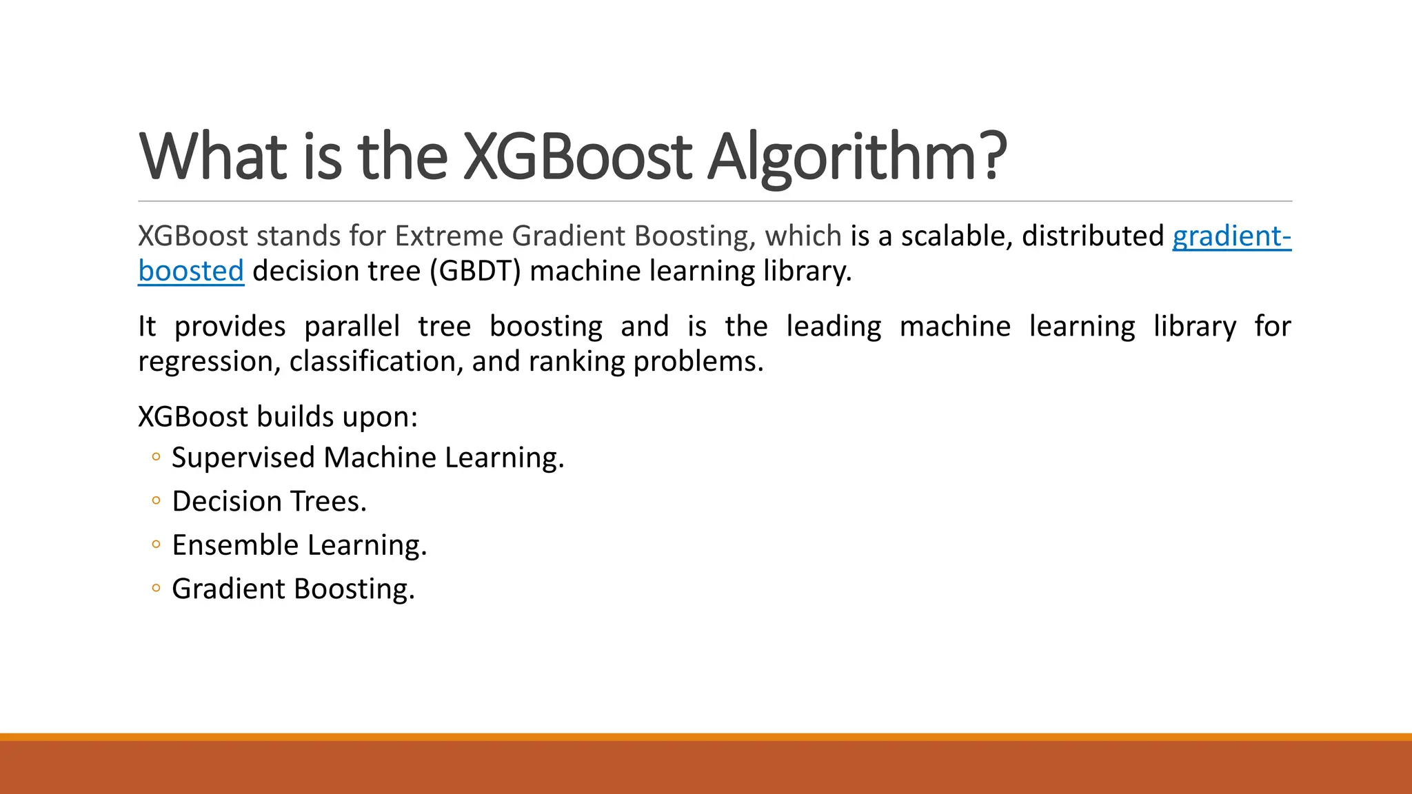
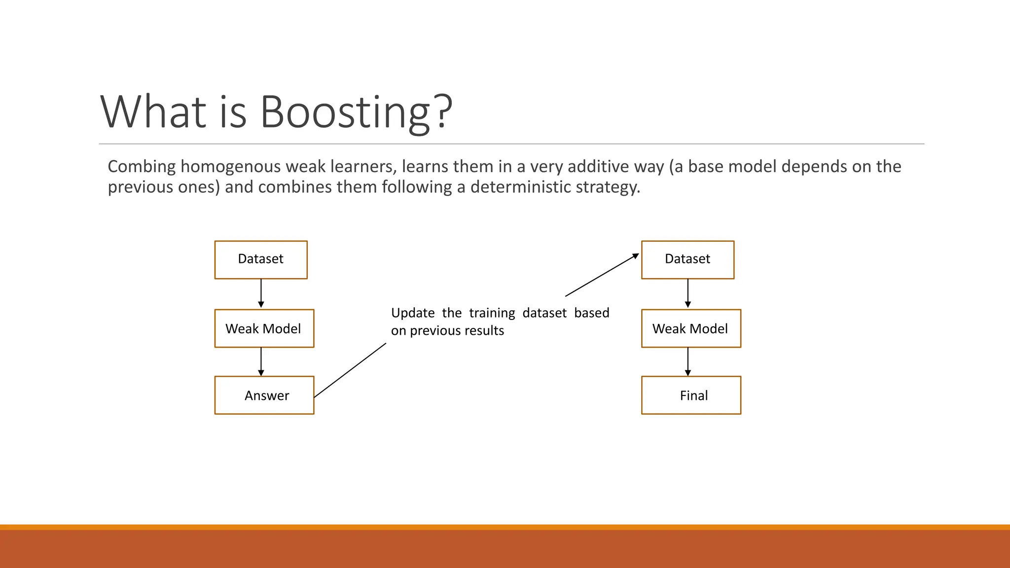
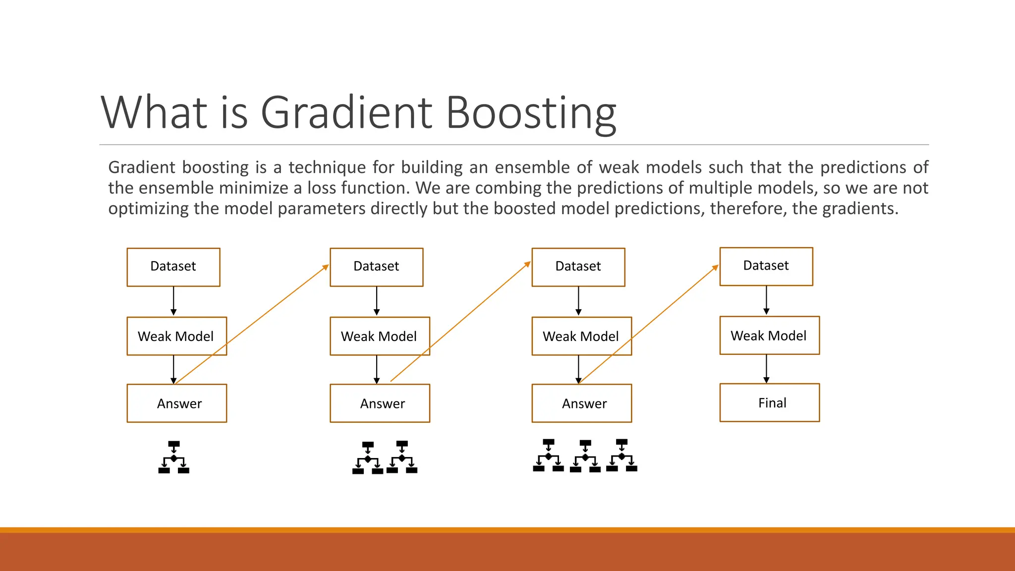
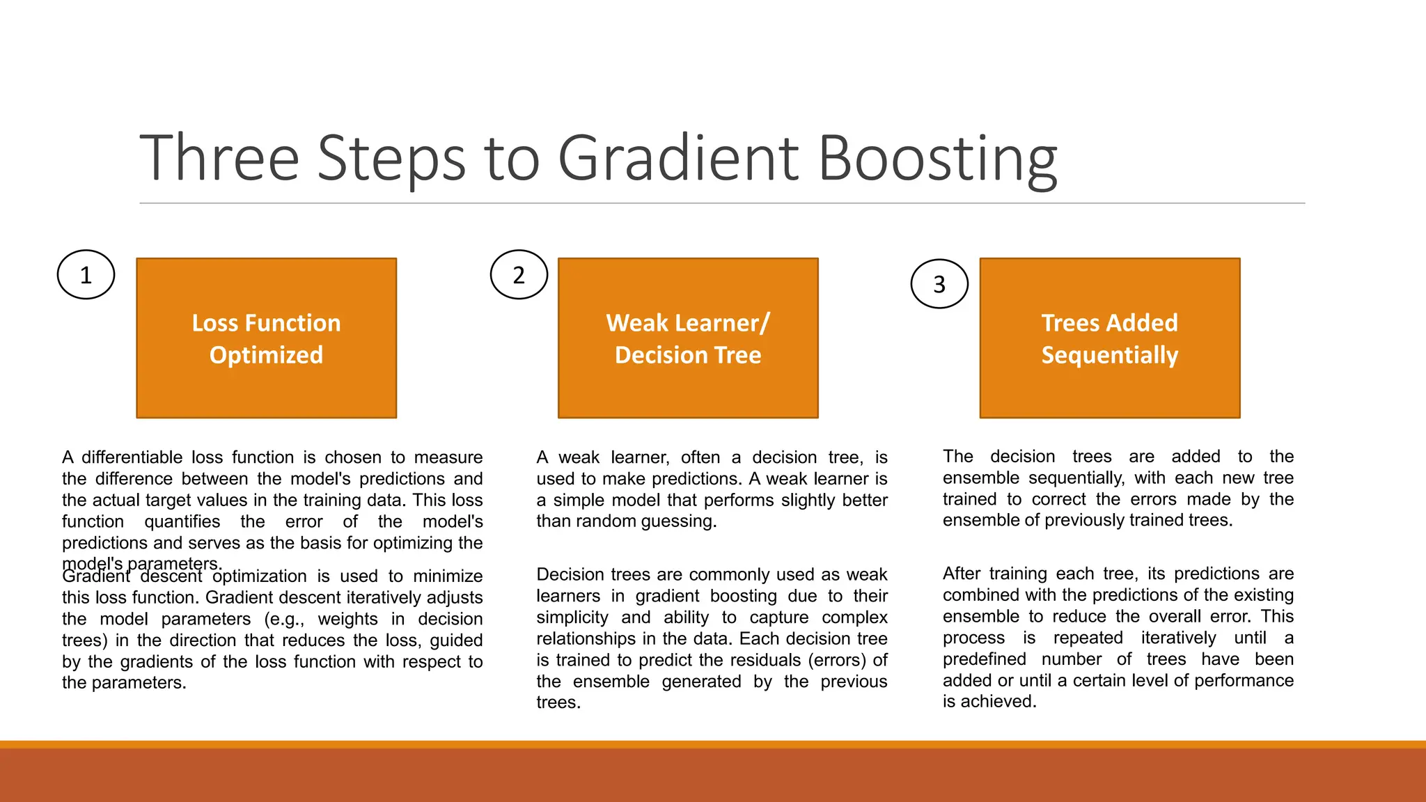
XGBoost is an advanced machine learning library for gradient-boosted decision trees, widely used for regression, classification, and ranking tasks. It uses principles of supervised learning, decision trees, and ensemble learning, specifically focusing on combining multiple weak models to enhance prediction accuracy. Key concepts include gradient boosting, loss function optimization, and the iterative process of adding decision trees to reduce overall error.

1. XGBoost
AGATHA LAU
25/4/2024

2. What is the XGBoost Algorithm?
XGBoost stands for Extreme Gradient Boosting, which is a scalable, distributed gradient-
boosted decision tree (GBDT) machine learning library.
It provides parallel tree boosting and is the leading machine learning library for
regression, classification, and ranking problems.
XGBoost builds upon:
◦ Supervised Machine Learning.
◦ Decision Trees.
◦ Ensemble Learning.
◦ Gradient Boosting.

3. Supervised Machine Learning
Supervised machine learning uses algorithms to train a model to find patterns in a
dataset with labels and features and then uses the trained model to predict the labels
on a new dataset’s features.
Figure 1: A supervised learning train a model to find pattern in a dataset and uses the trained model to predict labels on a new dataset.

4. Decision Trees
Decision trees create a model that predicts the label by evaluating a tree of if-then-else
true/false feature questions, and estimating the minimum number of questions needed
to assess the probability of making a correct decision.
Figure 2: A decision tree is used to estimate a house price (the label) based on the size and number of bedrooms (the features).

5. Ensemble Learning
A Gradient Boosting Decision Trees (GBDT) is a decision tree ensemble learning
algorithm similar to random forest, for classification and regression.
Ensemble models in Machine Learning combine the decisions from multiple models to
improve the overall performance.
Both random forest and GBDT build a model consisting of multiple decision trees. The
difference is in how the trees are built and combined.

6. Ensemble Methods
The principle behind ensembles is the idea of "wisdom of the crowd". The collective predictions
of many diverse models is better than any set of predictions made by a single model.
In ensemble learning theory, we call weak learners (base models) that can be used as building
blocks for designing more complex models by combining several of them.

7. What is Bagging?
Combing homogenous weak learners, learns them independently from each other in parallel and
combines them following some kind of deterministic averaging process.
Dataset
Samples
Samples
Samples
Weak Model
Weak Model
Weak Model
Ensemble

8. What is Boosting?
Combing homogenous weak learners, learns them in a very additive way (a base model depends on the
previous ones) and combines them following a deterministic strategy.
Dataset
Weak Model
Answer
Update the training dataset based
on previous results
Dataset
Weak Model
Final

9. What is Gradient Boosting
Gradient boosting is a technique for building an ensemble of weak models such that the predictions of
the ensemble minimize a loss function. We are combing the predictions of multiple models, so we are not
optimizing the model parameters directly but the boosted model predictions, therefore, the gradients.
Dataset
Weak Model
Answer
Dataset
Weak Model
Answer
Dataset
Weak Model
Answer
Dataset
Weak Model
Final

10. Three Steps to Gradient Boosting
Loss Function
Optimized
Weak Learner/
Decision Tree
Trees Added
Sequentially
A differentiable loss function is chosen to measure
the difference between the model's predictions and
the actual target values in the training data. This loss
function quantifies the error of the model's
predictions and serves as the basis for optimizing the
model's parameters.
Gradient descent optimization is used to minimize
this loss function. Gradient descent iteratively adjusts
the model parameters (e.g., weights in decision
trees) in the direction that reduces the loss, guided
by the gradients of the loss function with respect to
the parameters.
A weak learner, often a decision tree, is
used to make predictions. A weak learner is
a simple model that performs slightly better
than random guessing.
Decision trees are commonly used as weak
learners in gradient boosting due to their
simplicity and ability to capture complex
relationships in the data. Each decision tree
is trained to predict the residuals (errors) of
the ensemble generated by the previous
trees.
The decision trees are added to the
ensemble sequentially, with each new tree
trained to correct the errors made by the
ensemble of previously trained trees.
After training each tree, its predictions are
combined with the predictions of the existing
ensemble to reduce the overall error. This
process is repeated iteratively until a
predefined number of trees have been
added or until a certain level of performance
is achieved.
1 2 3

11. Summary
Defined Bagging and Boosting
Learned the Role of a Weak Learner
Defined Loss Function
Greedy Algorithm
Three Steps in Gradient Boosting
Learned about Ensembles