Ensembles.pdf

Leonardo Auslender Copyright 2004
Leonardo Auslender 1
Gradient Boosting and Comparative
Performance in Business Applications
DMA Webinar, 2017/03
Leonardo Auslender
Independent Statistical Consultant
Leonardo ‘dot’ Auslender ‘at’ Gmail ‘dot’ com.
Slides available at
https://independent.academia.edu/Auslender

Outline:
1) Why more techniques? Bias-variance tradeoff.
2)Ensembles
1) Bagging – stacking
2) Random Forests
3) Gradient Boosting (GB)
4) Gradient-descent optimization method.
5) Innards of GB.
6) Overall Ensembles.
7) Partial Dependence Plots (PDP)
8) Case Study.
9) Xgboost
10)On the practice of Ensembles.
11)References.
What is this webinar NOT about:
No software demonstration or training.

1) Why more techniques? Bias-variance tradeoff.
(Broken clock is right twice a day, variance of estimation = 0, bias extremely high.
Thermometer is accurate overall, but reports higher/lower temperatures at night.
Unbiased, higher variance. Betting on same horse always has zero variance, possibly
extremely biased).
Model error can be broken down into three components mathematically. Let f
be estimating function. f-hat empirically derived function.

Credit : Scott Fortmann-Roe (web)

Let X1, X2, X3,,, i.i.d random variables, usual mean and variance
Well known that variance E(X) =
By just averaging estimates, we lower variance and assure (‘hope’)
same aspects of bias since expected value of estimated mean is .
Let us find methods to lower or stabilize variance (at least) while
keeping low bias. And maybe even lower the bias.
Since trees (grown deep enough) are low-bias and high-variance,
shouldn’t we average trees somehow to lower variance?
 (high variance because if split data in half, and fit trees to each, predictions are usually very
different).
 And since no error can be fully attained, still searching for more techniques and giving
more lectures.
 Minimize general objective function (very relevant for XGBoost):
n
 
Minimize loss function to reduce bias.
Regularization, minimize model complexity.
Obj(Θ) L(Θ) Ω(Θ),
L(Θ)
Ω(Θ)
 


set of model parameters.
1 p
where Ω {w ,,,,,,w },


Ensembles.
Bagging (bootstrap aggregating, Breiman, 1996): Adding randomness 
improves function estimation. Variance reduction technique, reducing
also MSE. Let initial data size n.
1) Construct bootstrap sample by randomly drawing n times with replacement
(note, some observations repeated).
2) Compute sample estimator (logistic or regression, tree, ANN …).
3) Redo B times, B large (50 – 100 or more in practice).
4) Bagged estimator. For classification, Breiman recommends majority vote of
classification for each observation. Buhlmann (2003) recommends averaging
bootstrapped probabilities. Note that individual obs may not appear B times
each.
NB: This is independent sequence of trees. What if we remove independence? See next section.
Reduces prediction error by lowering variance of aggregated predictor
while maintaining bias almost constant (variance/bias trade-off).
Friedman (1998) reconsidered boosting and bagging in terms of
gradient descent algorithms.

Ensembles (cont. 1).
Evaluation:
Empirical studies: boosting yields (seen later) smaller
misclassification rates compared to bagging, reduction of
both bias and variance. Different boosting algorithms (Breiman’s
arc-x4 and arc-gv). In cases with substantial noise, bagging
performs better. Especially used in clinical studies.
Why does Bagging work?
Breiman: bagging successful because reduces instability of
prediction method. Unstable: small perturbations in data  large
changes in predictor. Experimental results show variance
reduction. Studies suggest that bagging performs some
smoothing on the estimates. Grandvalet (2004) argues that
bootstrap sampling equalizes effects of highly influential
observations.

Ensembles (cont. 2).
Adaptive Bagging (Breiman, 2001): Mixes bias-reduction boosting with
variance-reduction bagging. Uses out-of-bag obs to halt optimizer.
Stacking:
Previously, same technique used throughout. Stacking (Wolpert 1992)
combines different algorithms on single data set. Voting is then
used for final classification. Ting and Witten (1999) “stack” the
probability distributions (PD) instead.
Stacking is “meta-classifier”: combines methods.
Pros: takes best from many methods. Cons: un-interpretable, mixture
of methods become black-box of predictions.
Stacking very prevalent in WEKA.
NB: Trees and logistic Not Ensembles, but used later on in Overall
Ensemble technique.

2.2) L. Breiman:
Random Forests

Random Forests.
(Breiman, 2001) Decision Tree Forest: ensemble (collection) of
decision trees whose predictions are combined to make overall
prediction for the forest.
Similar to TreeBoost (Gradient boosting) model because large number
of trees are grown. However, TreeBoost generates series of trees with
output of one tree going into next tree in series. In contrast, decision
tree forest grows number of independent trees in parallel, and they
do not interact until after all of them have been built.
Disadvantage: complex model, cannot be visualized like single tree.
More “black box” like neural network  advisable to create both single-
tree and tree forest model (but see later for some help …).
Single-tree model can be studied to get intuitive understanding of how
predictor variables relate, and decision tree forest model can be used
to score data and generate highly accurate predictions.

Random Forests (cont. 1).
1. Random sample of N observations with replacement (“bagging”).
On average, about 2/3 of rows selected. Remaining 1/3 called “out
of bag (OOB)” obs. New random selection is performed for each
tree constructed.
2. Using obs selected in step 1, construct decision tree. Build tree to
maximum size, without pruning. As tree is built, allow only subset
of total set of predictor variables to be considered as possible
splitters for each node. Select set of predictors to be considered as
random subset of total set of available predictors.
For example, if there are ten predictors, choose five randomly as
candidate splitters. Perform new random selection for each split. Some
predictors (possibly best one) will not be considered for each split, but
predictor excluded from one split may be used for another split in same
tree.

Random Forests (cont. 3).
No Overfitting or Pruning.
"Over-fitting“: problem in large, single-tree models where model fits
noise in data  poor generalization power  pruning. In nearly all
cases, decision tree forests do not have problem with over-fitting, and no
need to prune trees in forest. Generally, more trees in forest, better fit.
Prediction: mode of collection of trees.
Internal Measure of Test Set (Generalization) Error .
About 1/3 of observations excluded from each tree in forest, called “out
of bag (OOB)”: each tree has different set of out-of-bag observations 
each OOB set constitutes independent test sample.
To measure generalization error of decision tree forest, OOB set for each
tree is run through tree and error rate of prediction is computed.

Leonardo Auslender 16 16

Detour: Underlying idea for boosting classification models (NOT yet GB).
(Freund, Schapire, 2012, Boosting: Foundations and Algorithms, MIT)
Start with model M(X) and obtain 80% accuracy, or 60% R2, etc.
Then Y = M(X) + error1. Hypothesize that error is still correlated with Y.
 error1 = G(X) + error2, where we model Error1 now, or
In general Error (t - 1) = Z(X) + error (t) 
Y = M(X) + G(X) + ….. + Z(X) + error (t-k). If find optimal beta weights to
combined models, then
Y = b1 * M(X) + b2 G(X) + …. + Bt Z(X) + error (t-k)
Boosting is “Forward Stagewise Ensemble method” with single data set,
iteratively reweighting observations according to previous error, especially focusing on
wrongly classified observations.
Philosophy: Focus on most difficult points to classify in previous step by
reweighting observations.

Main idea of GB using trees (GBDT).
Let Y be target, X predictors such that f 0(X) weak model to
predict Y that just predict mean value of Y. “weak” to avoid over-
fitting.
Improve on f 0(X) by creating f 1(X) = f 0(X) + h (x). If h perfect
model  f 1(X) = y  h (x) = y - f 0(X) = residuals = negative
gradients of loss functions.
Residual
fitting

Quick description of GB using trees (GBDT).
1) Create very small tree as initial model, ‘weak’ learner, (e.g., tree with two terminal nodes. (
 depth = 1). ‘WEAK’ avoids over-fitting and local minina, and predicts, F1, for each obs.
2) Each tree allocates a probability of event or a mean value in each terminal node, according
to the nature of the dependent variable or target.
3) Compute “residuals” (prediction error) for every observation (if 0-1 target, apply logistic
transformation to linearize them p / 1 – p).
4) Use residuals as new ‘target variable and grow second small tree on them (second stage of
the process, same depth). To ensure against over-fitting, use random sample without
replacement ( “stochastic gradient boosting”.)
5) New model, once second stage is complete, we obtain concatenation of two trees, Tree1 and
Tree2 and predictions F1 + F2 * gamma, gamma multiplier or shrinkage factor (called step
size in gradient descent).
6) Iterate procedure of computing residuals from most recent tree combination, which become
the target of the new model, and iterate.
7) In the case of a binary target variable, each tree produces at least some nodes in which
‘event’ is majority (‘events’ are typically more difficult to identify since most data sets
contain very low proportion of ‘events’ in usual case).
8) Final score for each observation is obtained by summing (with weights) the different scores
(probabilities) of every tree for each observation.

Why does it work?
Overfitting avoided by creating extremely simple trees. Bias fought
by searching for better fits.
Controls prediction variance by:
Limiting number of obs. in nodes.
Shrinkage regularization.
Limiting number of iterations by monitoring error rate on validation data
set.
Why “gradient” and “boosting”?
Gradient = residual,
Boosting due to iterative re-modeling of residuals.

More Details
Friedman’s general 2001 GB algorithm:
1) Data (Y, X), Y (N, 1), X (N, p)
2) Choose # iterations M
3) Choose loss function L(Y, F(x), Error), and corresponding gradient, i.e., 0-1 loss
function, and residuals are corresponding gradient. Function called ‘f’.
4) Choose base learner h( X, θ), say shallow trees.
Algorithm:
1: initialize f0 with a constant, usually mean of Y.
2: for t = 1 to M do
3: compute negative gradient gt(x), i.e., residual from Y as next target.
4: fit a new base-learner function h(x, θt), i.e., tree.
5: find best gradient descent step-size
6: update function estimate:
8: end for
(all f function are function estimates, i.e., ‘hats’).
0 <
n
t t t
i t 1 i i
γ i 1
, 1
γ argmin L(y ,f (x ) γh (x )) γ



 


 
t t 1 t t t
f f (x) γ h (x,θ )

Specifics of Tree Gradient Boosting, called TreeBoost (Friedman).
Friedman’s 2001 GB algorithm for tree methods:
Same as previous one, and
jt
prediction of tree t in final node N
for tree 'm'.
J
t jt jm
j 1
jt
h (x) p I(x N )
p :

 

t t-1
In TreeBoost Friedman proposes to find optimal
in each final node instead of
unique at every iteration. Then
f (x)=f (x)+
i jt
jm
J
jt t jt
j 1
jt i t 1 i t i
γ x N
,
γ h (x)I(x N ),
γ argmin L(y ,f (x ) γh (x ))
γ
γ,




 



Parallels with Stepwise (regression) methods.
Stepwise starts from original Y and X, and in later iterations
turns to residuals, and reduced and orthogonalized X matrix,
where ‘entered’ predictors are no longer used and
orthogonalized away from other predictors.
GBDT uses residuals as targets, but does not orthogonalize or
drop any predictors.
Stepwise stops either by statistical inference, or AIC/BIC
search. GBDT has a fix number of iterations.
Stepwise has no ‘gamma’ (shrinkage factor).

Setting.
Hypothesize existence of function Y = f (X, betas, error). Change of
paradigm, no MLE (e.g., logistic, regression, etc) but loss function.
Minimize Loss function itself, its expected value called risk. Many different
loss functions available, gaussian, 0-1, etc.
A loss function describes the loss (or cost) associated with all possible
decisions. Different decision functions or predictor functions will tend
to lead to different types of mistakes. The loss function tells us which
type of mistakes we should be more concerned about.
For instance, estimating demand, decision function could be linear equation
and loss function could be squared or absolute error.
The best decision function is the function that yields the lowest expected
loss, and the expected loss function is itself called risk of an estimator. 0-1
assigns 0 for correct prediction, 1 for incorrect.

Key Details.
Friedman’s 2001 GB algorithm: Need
1) Loss function (usually determined by nature of Y (binary,
continuous…)) (NO MLE).
2) Weak learner, typically tree stump or spline, marginally better
classifier than random (but by how much?).
3) Model with T Iterations:
# nodes in each tree;
L2 or L1 norm of leaf weights;
other. Function not directly
opti
T
t
i
t 1
n T
i i k
i 1 t 1
ŷ tree (X)
ˆ
Objective function : L(y , y ) Ω(Tree )
Ω {

 




 
mized by GB.}

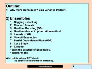
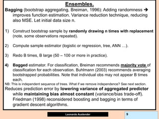
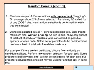
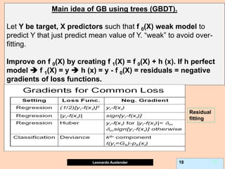
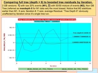
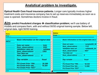
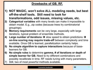
L2-error penalizes symmetrically away from 0, Huber penalizes less than OLS
away from [-1, 1], Bernoulli and Adaboost are very similar. Note that Y ε [-1, 1]
in 0-1 case here.

Visualizing GB, RF, Bagging …..
1) Via Partial Dependence plots to view variables relationships.
2) Approximate method: Create tree of posterior probabilities vs.
original predictors.

Gradient Descent.
“Gradient” descent method to find minimum of function.
Gradient: multivariate generalization of derivative of function in one
dimension to many dimensions. I.e., gradient is vector of partial
derivatives. In one dimension, gradient is tangent to function.
Easier to work with convex and “smooth” functions.
convex Non-convex

“Gradient” descent
Method of gradient descent is a first order optimization algorithm that is based on taking
small steps in direction of the negative gradient at one point in the curve in order to find
the (hopefully global) minimum value (of loss function). If it is desired to search for the
maximum value instead, then the positive gradient is used and the method is then called
gradient ascent.
Second order not searched, solution could be local minimum.
Requires starting point, possibly many to avoid local minima.

Leonardo Auslender 32 Ch. 5-32
Comparing full tree (depth = 6) to boosted tree residuals by iteration..
2 GB versions: 1) with raw 20% events (M1), 2) with 50/50 mixture of events (M2). Non GB
Tree (referred as maxdepth 6 for M1 data set) the most biased. Notice that M2 stabilizes
earlier than M1. X axis: Iteration #. Y axis: average Residual. “Tree Depth 6” obviously
unaffected by iteration since it’s single tree run.
1.5969917399003E-15
-2.9088316687833E-16
Tree depth 6 2.83E-15
0 2 4 6 8 10
Iteration
-5E-15
-2.5E-15
0
2.5E-15
5E-15
MEAN_RESID_M1_TRN_TREES
Avg residuals by iteration by model names in gradient boosting
Vertical line - Mean stabilizes

Comparing full tree (depth = 6) to boosted tree residuals by iteration..
Now Y = Var. of resids. M2 has highest variance followed by Depth 6 (single tree) and
then M1. M2 stabilizes earlier as well. In conclusion, M2 has lower bias and higher variance
than M1 in this example, difference lies on mixture of 0-1 in target variable.
0.1218753847
8
0.1781230782
5
Depth 6 = 0.145774
0.1219
0.1404
0.159
0.1775
0.196
0.2146
Var
of
Resids
0 2 4 6 8 10
Iteration
VAR_RESID_M2_TRN_TREES
VAR_RESID_M1_TRN_TREES
Variance of residuals by iteration in gradient boosting
Vertical line - Variance stabilizes

Overall Ensembles.
Given specific classification study and many different modeling techniques,
create logistic regression model with original target variable and the
different predictions from the different models, without variable selection (this
is not critical). Alternatively, run Regression Tree.
Since ranges of different predictions may differ, first apply Platt’s
normalization to each model predictions (logistic regression).
Evaluate importance of different models either via p-values or partial
dependence plots.
Note: It is not similar to Bagging, Stacking, etc, because does not use
VOTING.

Comparing Ensemble Methods I.
Bagging and RF
Bagging: single parameter, number of trees. All trees are fully grown
binary tree (unpruned) and at each node in the tree one searches over all
features to find feature that best splits the data at that node.
RF has 2 parameters: 1: number of trees. 2: mtry, number of features to
search over to find best split, typically p/3 for regression, SQRT(p) or log2(p)
for classification. Thus during tree creation randomly mtry number of
features are chosen from all available features and best feature that splits
the data is chosen.
RF lowers variance by reducing correlation among trees, accomplished
by random selection of feature-subset for split at each node. In Bagging
case, if there’s strong predictor, likely will be top split and most trees will be
highly correlated, but not so with RF.

Leonardo Auslender Copyright 2004 Ch. 5-37
Comparing Ensemble Methods II.
GB learns slowly and no bootstrapped samples but sequence of trees
based on sequential residuals as target on original sample. 3 parameters:
1. # trees. If too large, can overfit, can be selected by cross-validation or
outside validation sample.
2. Shrinkage parameter lambda, controls boosting learning.
3. Tree depth, usually stumps.
Claim :
Trees Bagging Random Forest Gradient Boosting

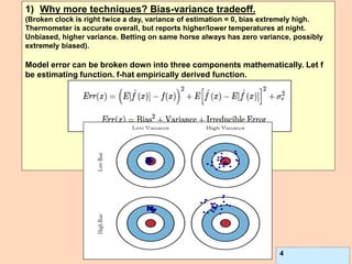
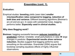
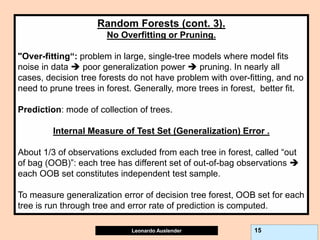
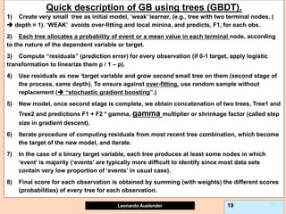
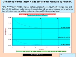
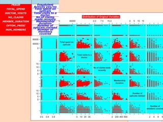
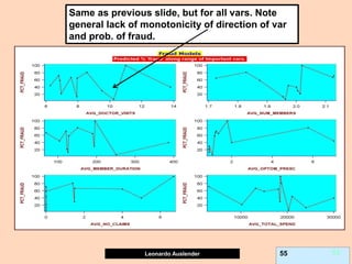
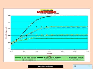
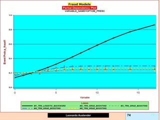
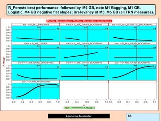
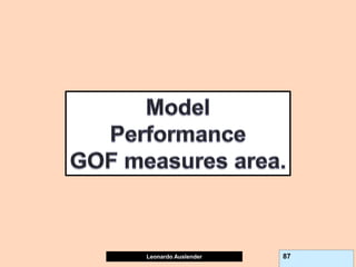
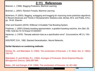
Partial Dependence plots (PDP).
Due to GB (and other methods’) black-box nature, PDPs show effect of predictor X on
fitted modeled response (notice, NOT ‘true’ model values) once all other predictors
have been marginalized (integrated away). Marginalized Predictors usually fixed at
constant value, such as mean. Graphs may not capture nature of variable interactions
especially if interaction significantly affect model outcome.
Assume Y = f (X) = f (Xa, Xb), where X = Xa U Xb, Xa subset of predictors of interest. PDP
displays the marginal expected value of f (Xa), by averaging over values of Xb (and
assuming Xa to be single predictor), given by f(Xa = xa, Avg (Xbi))) where the average of
the function for a given value (vector) of the subset Xa is the average value of the model
output setting the Xa to value of interest and averaging the result with the values of Xb as
they exist in the data set. Formally:
Since GB, Boosting, Bagging, etc are BLACK BOX models, use PDP to obtain model
interpretation. Also useful for logistic models.
b
b
b b
X a b a b b
X
a a a b
x X
b
E [f(X , X )] f(X , X )dP(X ),
P : unknown density. Integral estimated by :
1
PDP(X x ) f(x , x )
| X | 

 



PDP Usefulness.
1) Specific predictor effect on fitted model: for instance, in credit
card default models, ascertain effect of tenure length on fitted model. Or, in loan
models, whether advanced age negatively affects loaning.
2) Control variables: In epidemiological studies, dose response is important.
PDP would provide info about optimal dose levels. In click through prediction, could
provide info on optimal length of message to enhance click through rate.
3) Can be used to visualize two-way interactions: Notice that in previous formula,
Xa can be more than one predictor.

Analytical problem to investigate.
Optical Health Care fraud insurance patients. Longer care typically involves higher
treatment costs and insurance company has to set up reserves immediately as soon as a
case is opened. Sometimes doctors involve in fraud.
Aim: predict fraudulent charges  classification problem; we’ll use battery of
models and compare them, with and without 50/50 original training sample. Below left,
original data, right 50/50 training.
Notice
1
From .....
**************************************************************** 1
................. Basic information on the original data
set.s: 1
................. ..
1
................. Data set name ........................ train 1
................. Num_observations ................ 3595 1
................. Validation data set ................. validata 1
................. Num_observations .............. 2365 1
................. Test data set ................ 1
................. Num_observations .......... 0 1
................. ... 1
................. Dep variable ....................... fraud 1
................. ..... 1
................. Pct Event Prior TRN............. 20.389 1
................. Pct Event Prior VAL............. 19.281 1
................. Pct Event Prior TEST ............ 1
*************************************************************
**** 1
Notice
1
From .....
****************************************************************
1
................. Basic information on the original data set.s:
1
................. ..
1
................. Data set name ........................ sampled50_50
1
................. Num_observations ................ 1133
1
................. Validation data set ................. validata50_50
1
................. Num_observations .............. 4827
1
................. Test data set ................
1
................. Num_observations .......... 0
1
................. ...
1
................. Dep variable ....................... fraud
1
................. .....
1
................. Pct Event Prior TRN............. 50.838
1
................. Pct Event Prior VAL............. 12.699
1
................. Pct Event Prior TEST ............
1
*****************************************************************
1

FRAUD Fraudulent
Activity yes/no
TOTAL_SPEND Total spent on
opticals
DOCTOR_VISITS Total visits to a
doctor
NO_CLAIMS No of claims
made recently
MEMBER_DURATION Membership
duration
OPTOM_PRESC Number of
opticals claimed
NUM_MEMBERS Number of
members
covered

Comment on Fraud Models.
Data set extremely simplified for illustration purposes.
In addition, difficult to ascertain fraudsters’ behavior, which
is known to change in order not to be discovered. Thus,
financial fraud amounts not necessarily large for single
claims, but divided into many claims 
Financial charts below may not show full fraudster ranking.
Further, if interest centers on ‘amount’, then possible better
model is two-stage model (Heckman, 1979).

Additional Information: Logistic backwards, RF and Trees for M1 only,
M1 – M6 for GB, all models evaluated at TRN and VAL stages. Naming convention:
M#_modeling.Method and sometimes M#_TRN/VAL_modeling.method. Also, run
Bagging at M1 but reporting only on AUROC to avoid clutter. M1 – M6 focuses on
changing depth of trees and iterations for GB, with p = 6 predictors.
For instance, M1_logistic_backward means Case M1 that uses logistic regression
with backward selection.
Ensemble: take all model predictions at end of M6 as predictors and run BACKWARD
logistic (or any other var sel) against actual dependent variable, and report 
ENSEMBLING by probability.
Requested Models: Names & Descriptions Model #
Model Name Model Description
***
Overall Models
M1 Raw DATA 20 pct maxdepth 1 num iterations 3
-2
-2
-2
-2
-2
-2
Compare GB in different settings with Logistic, Bagging, RF
(implicit regularization in Iterations and depth).

Methods utilized
Logistic regression, backward selection.
Classification Trees.
Bagging
Gradient Boosting (in different flavors, detailed by M1-M6)
Random Forests (defaults: train fraction = 0.6, # vars to search: 2, max depth: 50
max trees 10
Overall Ensemble

Significance except
Possibly for
doctor_visits.

No-event Event --- M1_TRN_TREES
M1 tree (illustration purposes).
To be compared with GB models later on. Larger
depth very difficult to visualize. Variables selected
agree with significant vars selected by Logistic.

2 most important vars.
Note: almost parallel loess
curves.

Final nodes along range of No_claims. Blue-
dashed lines: fraud nodes. Notice clumping at 0
no_claims, and non-fraud node at no_claims
between 4 and 6

Same as previous slide, but for all vars. Note
general lack of monotonicity of direction of var
and prob. of fraud.

Gains Table
% Resp.
Cum %
Resp
% Capt.
Resp.
Cum %
Capt.
Resp. Lift Cum Lift
Brier
Score *
100
Pctl Min
Prob
Max
Prob
Model Name
29.88 49.55 14.63 48.60 1.47 2.43 20.95
20 0.298 0.298 M1_TRN_TREES
M1_VAL_TREES 34.15 44.82 17.67 46.49 1.77 2.32 22.67
30 0.217 0.298 M1_TRN_TREES 24.97 41.35 12.26 60.87 1.22 2.03 18.57
M1_VAL_TREES 26.33 38.65 13.69 60.18 1.37 2.00 19.14
40 0.217 0.217 M1_TRN_TREES 21.73 36.45 10.64 71.51 1.07 1.79 17.01
M1_VAL_TREES 22.20 34.54 11.49 71.66 1.15 1.79 17.27
50 0.131 0.217 M1_TRN_TREES 15.96 32.35 7.84 79.34 0.78 1.59 13.25
M1_VAL_TREES 13.38 30.30 6.96 78.62 0.69 1.57 11.46
60 0.131 0.131 M1_TRN_TREES 13.11 29.14 6.42 85.76 0.64 1.43 11.39
M1_VAL_TREES 11.75 27.22 6.08 84.70 0.61 1.41 10.39
70 0.061 0.131 M1_TRN_TREES 10.49 26.48 5.15 90.91 0.51 1.30 9.28
M1_VAL_TREES 8.92 24.60 4.64 89.34 0.46 1.28 8.08
80 0.061 0.061 M1_TRN_TREES 6.18 23.94 3.03 93.94 0.30 1.17 5.80
M1_VAL_TREES 6.86 22.39 3.55 92.89 0.36 1.16 6.39
90 0.061 0.061 M1_TRN_TREES 6.18 21.97 3.03 96.97 0.30 1.08 5.80
M1_VAL_TREES 6.86 20.66 3.56 96.45 0.36 1.07 6.39
100 0.061 0.061 M1_TRN_TREES 6.18 20.39 3.03 100.00 0.30 1.00 5.80
M1_VAL_TREES 6.86 19.28 3.55 100.00 0.36 1.00 6.39

Comparing Gains-chart info with Precision Recall.
The gains-chart provides information on cumulative # of
Events per descending percentile / bin of probs. These bins
contain a fixed number of observations.
Precision recall instead is at probability level, not at bin
Level, and thus # of observations along the curve is not
Uniform. Thus, selecting cutoff point from gains-chart selects
invariably from within a range of probabilities.
Selecting from Precision recall, selects a specific probability
point.

Similar for 50/50. Random Forests and Grad Boosting differ
In variable importance values but not rankings. Notice that
Doctor_visits is used by GB and RF.

As we increase # iterations and maximum depth, larger
Number of variables selected. For RF, importance
Measured as rescaling of Gini, last var (num_members)
Dropped.

50/50: trees
Seriously
Affected,
Not so GB.
RF omitted.

Models insignificant except for M6_grad_Boosting.

50/50: scales
Shifted up.

Very interesting almost U relationship, conditioned on
Other vars in model.

M1_BG_TRN_TREES
No-event Event M1_BG_TRN_TREES
Divergence from trees in
Third level, e.g., member_duration 127.5
Versus No_Claims 4.5 from trees.

M1_GB_TRN_TREES
No-event Event M1_GB_TRN_TREES
GB model for M1

M3_GB_TRN_TREES
Original Tree splits on 1_no_claims 0.5,
2_member_duration 180.5 and 3_no_claims
3.5.
GB model M3

M6_GB_TRN_TREES
GB model M6.
Notice difference
with GB M3.

M1_RF_TRN_TREES
No-event Event M1_RF_TRN_TREES
Random Forests. It starts
With no_claims at 0.5 but
Then it jumps to total_spend.

Some quick comparison among Trees, GB and RF.
The 3 methods start with No_claims at 0.5. RF can’t do
its random predictor selection successfully because
there are few predictors to begin with.
In 2nd level, we notice divergence. RF jumps to
total_spend (4600 and 13950), GB splits on No_claims
(4.5) and Total_spend (5150), while trees at no_claims
(3.5) and member_duration (180.5).
Trees and Bagging diverse in 3rd level as seen, and
obviously bagging diverges from GB and RF.
From there on, the divergences obviously increase.

R_Forests best performance, followed by M6 GB, note M1 Bagging, M1 GB,
Logistic, M4 GB negative flat slopes; irrelevancy of M3, M5 GB (all TRN measures).

Probs shifted up for 50/50. Note different ranges, need to normalize.

GB, RF do not over-fit. If
selecting by Auroc, use GB or
RF.

50/50: overall ranking hasn’t changed. Notice
Decline in Trees, and stability in bagging.
Some evidence of over-
fitting. RF omitted.

50/50 Ranking Same.
RF poor VAL, great
TRN. Ensemble great.

(Cheating a bit, added Naive Bayes).
Methods similar in
financial performance.

XGBoost
Developed by Chen and Guestrin (2016) XGBoost: A Scalable Tree
Boosting System.
Claims: Faster and better than neural networks and Random Forests.
More efficient than GB due to parallel computing on single computer
(10 times faster). Algorithm takes advantage of advanced
decomposition of objective function that allows for outperforming
GB.
Not yet SAS available. Available in R, Julia, Python, CLI.
Tool used in many champion models in recent competitions (Kaggle,
etc.).

General Comments I.
1) Not immediately apparent what weak classifier is for GB (e.g., by
varying depth in our case). Likewise, number of iterations is big
issue. In our simple example, M6 GB was best performer, but
performance could worsen with larger # iterations. Still, overall
modeling benefited from ensembling all methods as measured by
either Cum Lift or ensemble p-values.
2) The posterior probability ranges are vastly different and thus the
tendency to classify observations by the .5 threshold is too simplistic.
3) PDPs show that different methods find distinct multivariate structures.
Interestingly, ensemble p-values show a decreasing tendency by
logistic and trees and a strong S shaped tendency by M6 GB,
which could mean that M6 GB alone tends to overshoot its
predictions.
4) GB relatively unaffected by 50/50 mixture.

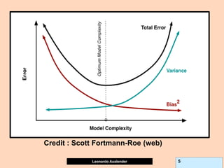
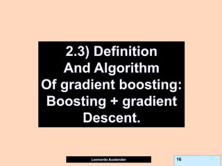
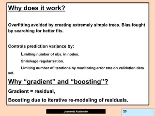
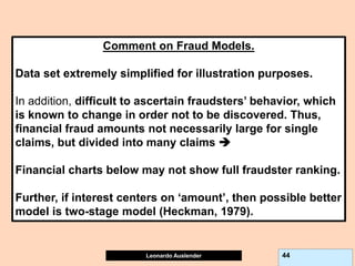
General Comments II.
5) While on classification GB problems, predictions are within [0, 1], for
continuous target problems, predictions can be beyond the range of the
target variable  headaches. I.e., negative predictions for target > 0.
This is due to the fact that GB models residuals at each iteration, not the
original target; this can lead to surprises, such as negative predictions
when Y takes only non-negative values, contrary to the original Tree
algorithm.
6) GB Shrinkage parameter and early stopping (# trees) act as
regularizers but combined effect not known and could be ineffective.
7) If GB shrinkage too small, and allow large Tree, model is large,
expensive to compute, implement and understand.
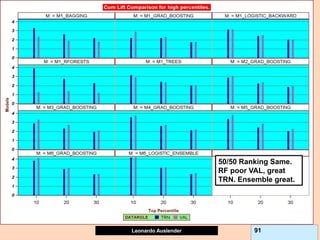
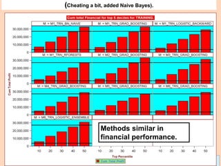
8) Financial Information not easily ranked. Ranking models according to
financials not equivalent to rankings by fraud detection (i.e., cum lift).

General Comments III.
9) Impossible to determine ‘best’ model without fully defined objective.
Overall ensemble p-values show M6_GB, financials show good Bagging
performance (and Naive Bayes, not shown).
10) Probably important to better understand patterns found by GB and
RF to obtain more comprehensive model/s and how each balances trade-
off of bias vs variance.

Drawbacks of GB, RF.
1) NOT MAGIC, won’t solve ALL modeling needs, but best
off-the-shelf tools. Still need to look for
transformations, odd issues, missing values, etc.
2) Categorical variables with many levels can make it impossible to
obtain model. E.g., zip codes (because trees try combinatorial
groupings).
3) Memory requirements can be very large, especially with large
iterations, typical problem of ensemble methods.
4) Large number of iterations  slow speed to obtain predictions 
on-line scoring may require trade-off between complexity and time
available. Once GB is learned, parallelization certainly helps.
5) No simple algorithm to capture interactions because of base-
learners for GB.
6) No simple rules to determine gamma, # of iterations or depth of
simple learner for GB. Need to try different combinations and
possibly recalibrate in time. RF needs tuning with many parameters.
7) Still, two of most powerful methods available.

2.11) References
Breiman, L. (1996): Bagging Predictors, Machine Learning.
Breiman, L. (2001): Random Forests, Machine Learning.
Bühlmann, P. (2003). Bagging, subagging and bragging for improving some prediction algorithms.
In Recent Advances and Trends in Nonparametric Statistics (eds. Akritas, M.G. and Politis, D.N.),
pp. 19-34. Elsevier.
Chen and Guestrin (2016): XGBoost: A Scalable Tree Boosting System.
Friedman, J. (2001).Greedy boosting approximation: a gradient boosting machine. Ann.Stat. 29,
1189–1232.doi:10.1214/aos/1013203451
Heckman, J. (1979). "Sample selection bias as a specification error". Econometrica. 47 (1): 153–
61.
WOLPERT, D.H., 1992. Stacked Generalization. Neural Networks.
Earlier literature on combining methods:
Winkler, RL. and Makridakis, S. (1983). The combination of forecasts. J. R. Statis. Soc. A. 146(2),
150-157.
Makridakis, S. and Winkler, R.L. (1983). Averages of Forecasts: Some Empirical Results,.
Management Science, 29(9) 987-996.
Bates, J.M. and Granger, C.W. (1969). The combination of forecasts. Or, 451-468.

Ensembles.pdf

More Related Content

Similar to Ensembles.pdf

More from Leonardo Auslender

Recently uploaded

Ensembles.pdf