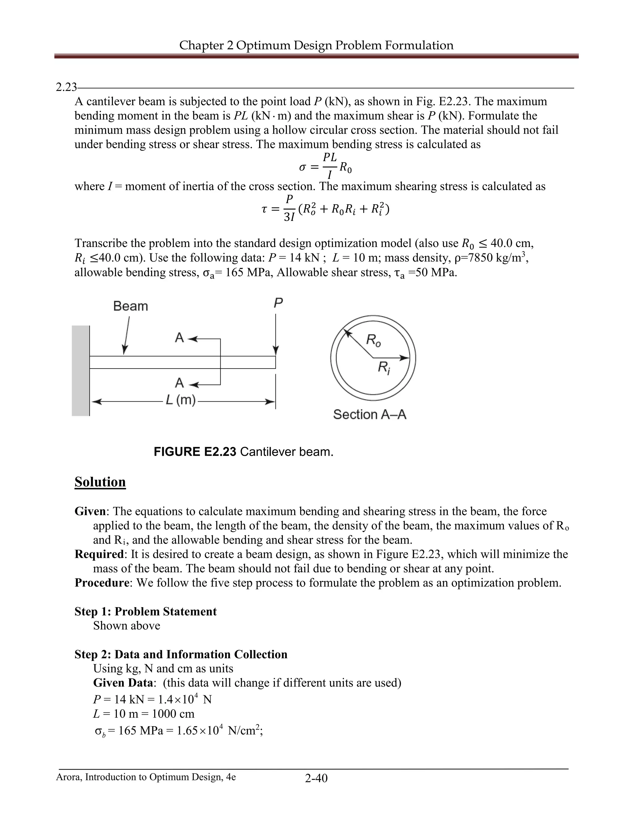
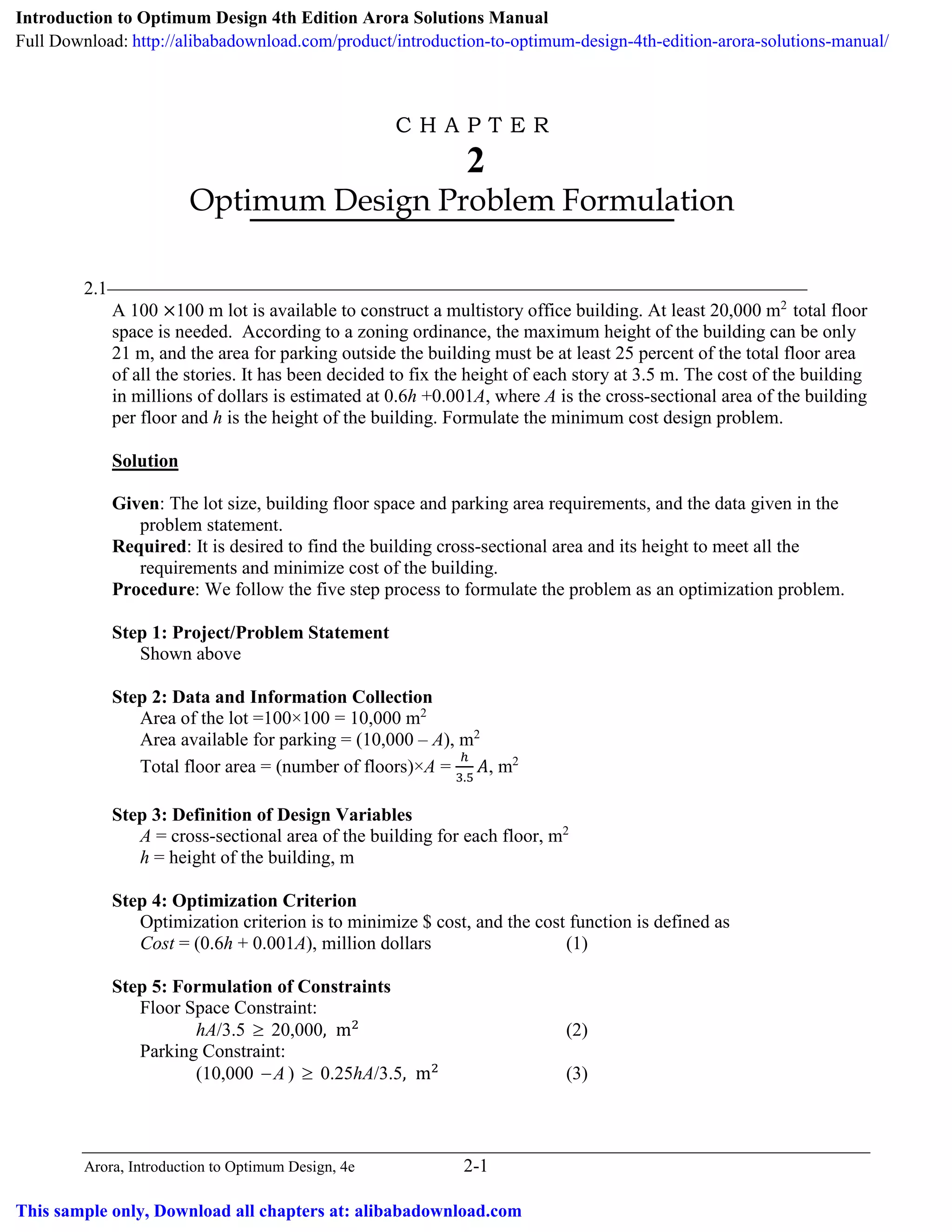
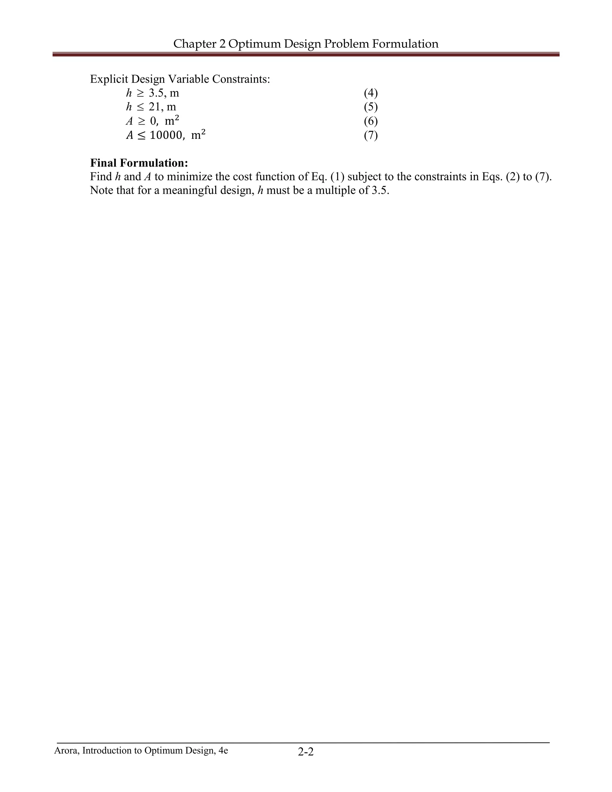
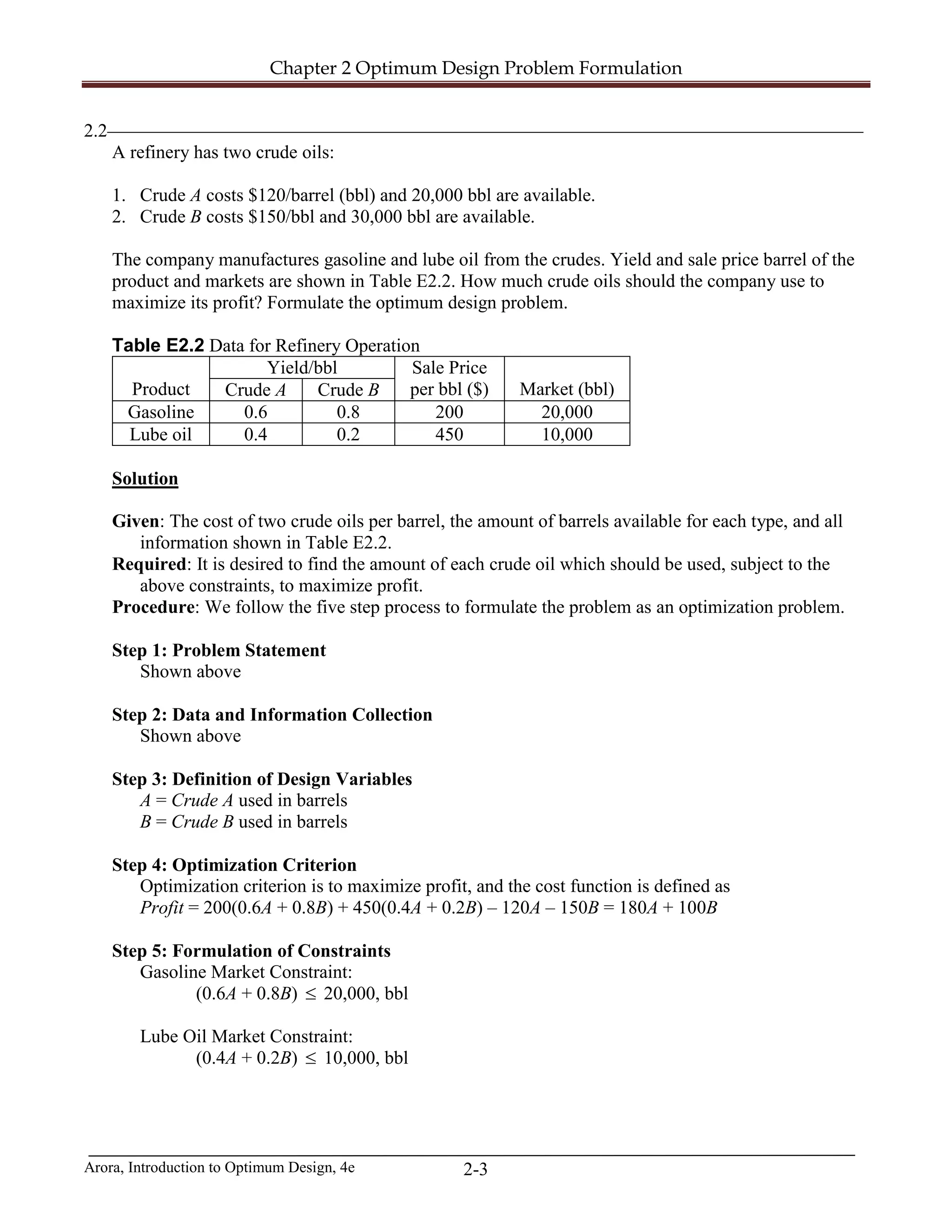
The document details various optimization design problems, including constructing a multistory office building, refining crude oils for maximum profit, designing a beer mug, and optimizing a heat exchanger's tube dimensions. Each problem follows a structured five-step process involving a project statement, data collection, variable definitions, optimization criteria, and constraints formulation. The goal across these examples is to minimize costs or maximize profits while adhering to various design limitations.

![Chapter 2 Optimum Design Problem Formulation
Arora, Introduction to Optimum Design, 4e 2-38
1
1 1
1 1
2
( 2 )
( )
2 2
H
H w
H w w sf
+
+
= =
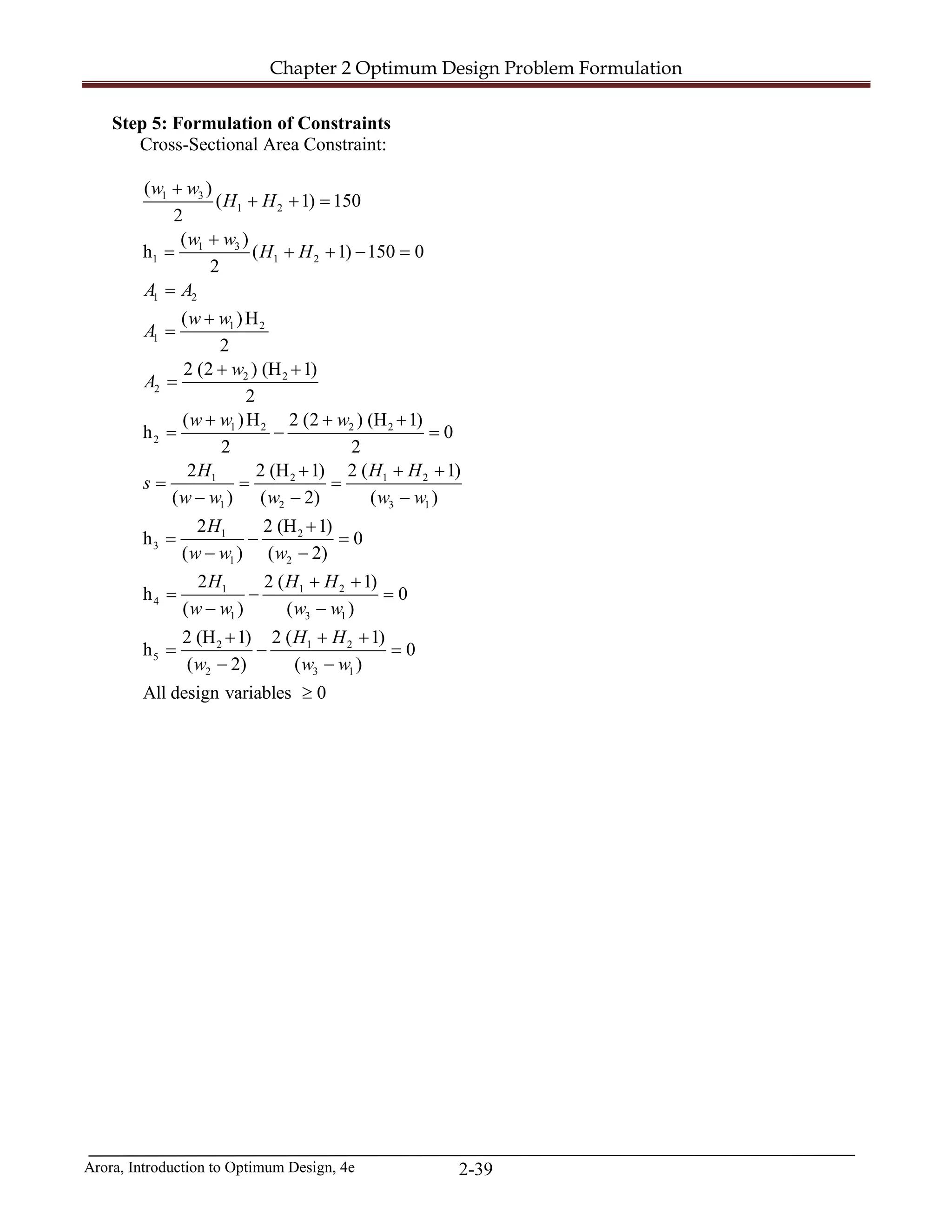
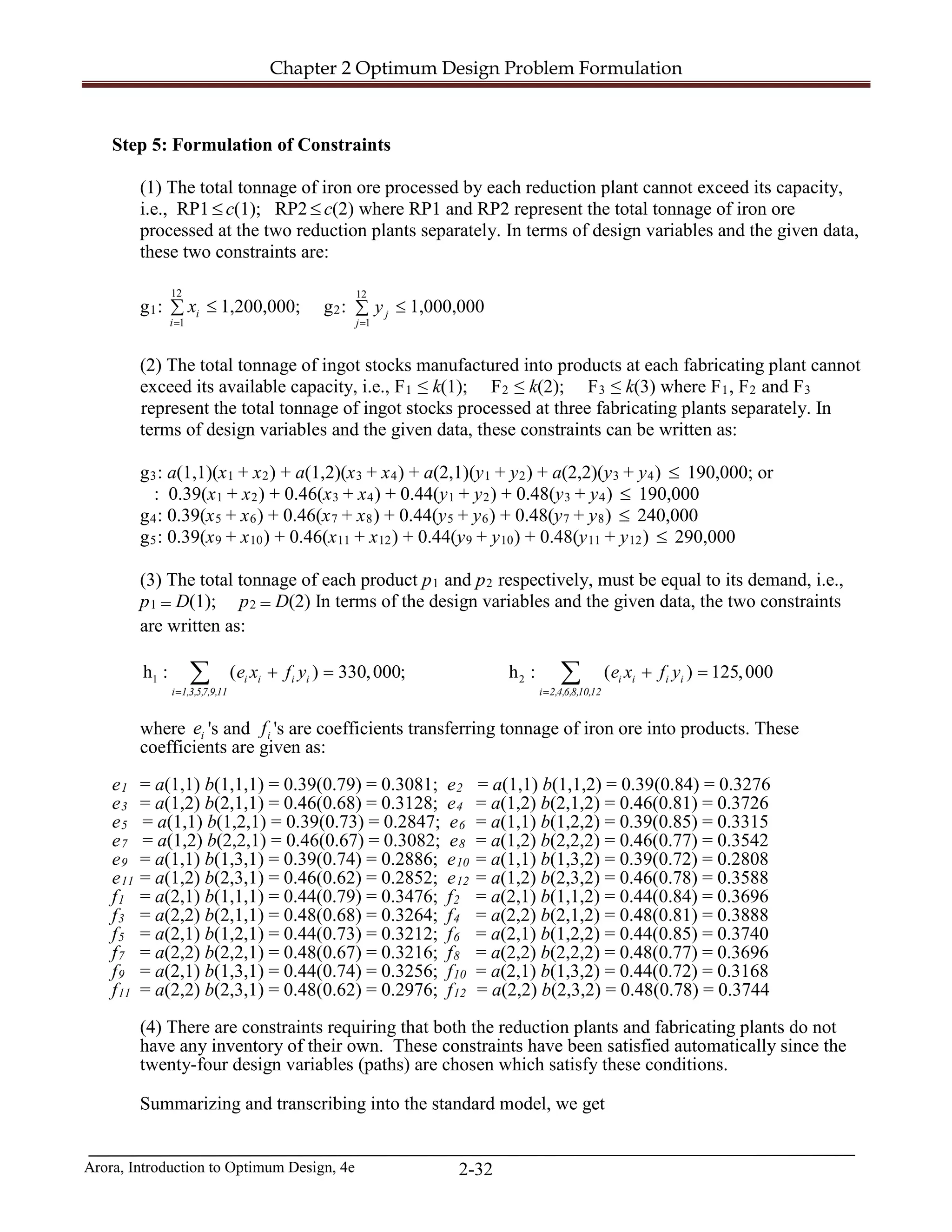
Step 5: Formulation of Constraints
Cross-Sectional Area Constraint:
1 3
1 2
1 2
1
1 1 2
1 2
1
1 1
2 2
2
1 1 2
( )
( 1) 150
2
2 ( 1)
[2 ]
h *( 1) 150 0
2
2
(2 )
2 (H 1)(2 2 2 ( 1)
h 0
2 2
All design variables must be non-negative :
, , , 0
w w
H H
H H
w
s H H
A A
H
H w
Hs
w H H s
+
+ + =
+ +
+
+ + −=
=
+
+ + + +
= − =
≥
Formulation 3:
Step 1: Problem Statement
Shown above
Step 2: Data and Information Collection
Shown above
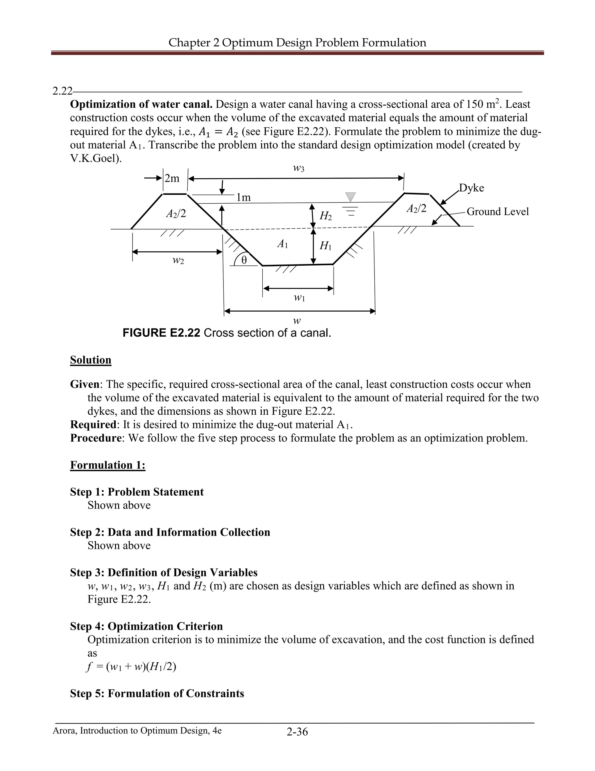
Step 3: Definition of Design Variables
A1, A2, w, w1, w2, w3, H1, H2 (m), and s (unitless) are chosen as design variables which are
defined above in Figure E2.22 and below:
tans θ=
Step 4: Optimization Criterion
Optimization criterion is to minimize the volume of excavation, and the cost function is defined
as:
1f A=](https://image.slidesharecdn.com/introduction-to-optimum-design-4th-edition-arora-solutions-manual-190412110526/75/Introduction-to-Optimum-Design-4th-Edition-Arora-Solutions-Manual-38-2048.jpg)