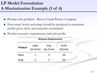
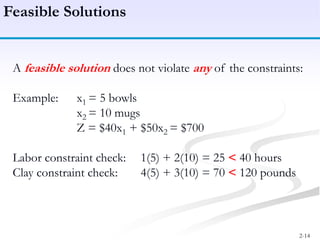
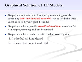
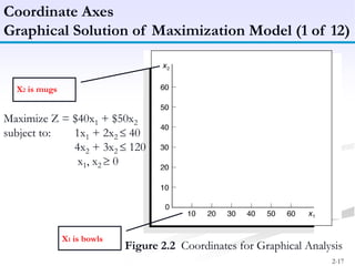
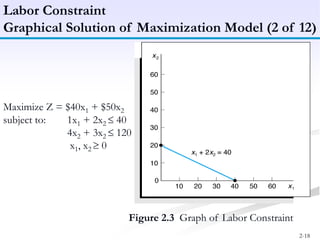
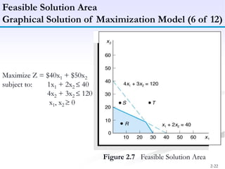
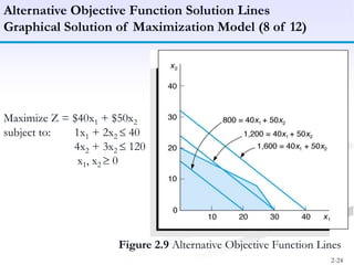
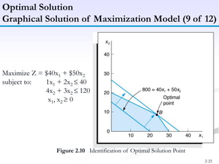
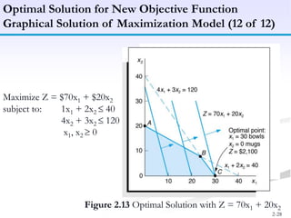
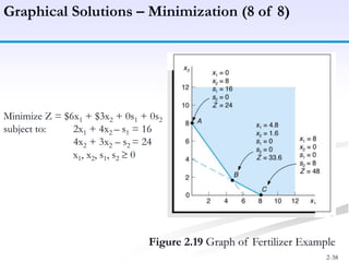
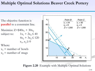
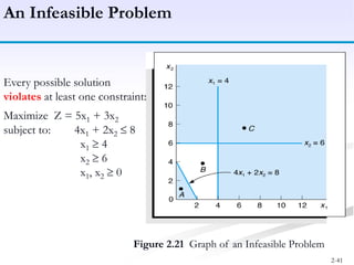
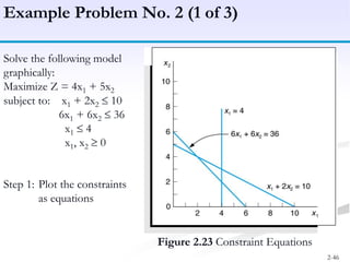
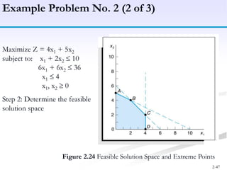
The document discusses linear programming models for solving business optimization problems. It provides an overview of linear programming and the steps to formulate a linear programming model, which are to define decision variables, construct the objective function, and formulate constraints. The document also discusses graphical solutions to linear programming problems using examples of maximizing profit from two products given resource constraints and minimizing fertilizer costs given nutrient requirements.

1. 2-1
Linear Programming:
Model Formulation and
Graphical Solution
JOSEPH GEORGE KONNULLY
Prepared by

2. 2-2
Topics
 Linear Programming – An overview
 Model Formulation
 Characteristics of Linear Programming Problems
 Assumptions of a Linear Programming Model
 Advantages and Limitations of a Linear Programming.
 A Maximization Model Example
 Graphical Solutions of Linear Programming Models
 A Minimization Model Example
 Irregular Types of Linear Programming Models

3. 2-3
 Objectives of business decisions frequently involve
maximizing profit or minimizing costs.
 Linear programming uses linear algebraic relationships
to represent a firm’s decisions, given a business objective,
and resource constraints.
 Steps in application:
1. Identify problem as solvable by linear programming.
2. Formulate a mathematical model of the unstructured
problem.
3. Solve the model.
4. Implementation
Linear Programming: An Overview

4. 2-4
 Decision variables - mathematical symbols representing levels
of activity of a firm.
 Objective function - a linear mathematical relationship
describing an objective of the firm, in terms of decision variables
- this function is to be maximized or minimized.
 Constraints – requirements or restrictions placed on the firm by
the operating environment, stated in linear relationships of the
decision variables.
 Parameters - numerical coefficients and constants used in the
objective function and constraints.
Model Components

5. 2-5
Summary of Model Formulation Steps
Step 1 : Clearly define the decision variables
Step 2 : Construct the objective function
Step 3 : Formulate the constraints

6. 2-6
Characteristics of Linear Programming Problems
 A decision amongst alternative courses of action is required.
 The decision is represented in the model by decision variables.
 The problem encompasses a goal, expressed as an objective
function, that the decision maker wants to achieve.
 Restrictions (represented by constraints) exist that limit the
extent of achievement of the objective.
 The objective and constraints must be definable by linear
mathematical functional relationships.

7. 2-7
 Proportionality - The rate of change (slope) of the objective
function and constraint equations is constant.
 Additivity - Terms in the objective function and constraint
equations must be additive.
 Divisibility -Decision variables can take on any fractional value
and are therefore continuous as opposed to integer in nature.
 Certainty - Values of all the model parameters are assumed to
be known with certainty (non-probabilistic).
Assumptions of Linear Programming Model

8. 2-8
 It helps decision - makers to use their productive resource
effectively.
 The decision-making approach of the user becomes more
objective and less subjective.
 In a production process, bottle necks may occur. For example, in
a factory some machines may be in great demand while others
may lie idle for some time. A significant advantage of linear
programming is highlighting of such bottle necks.
Advantages of Linear Programming Model

9. 2-9
 Linear programming is applicable only to problems where the
constraints and objective function are linear i.e., where they can
be expressed as equations which represent straight lines. In real
life situations, when constraints or objective functions are not
linear, this technique cannot be used.
 Factors such as uncertainty, and time are not taken into
consideration.
 Parameters in the model are assumed to be constant but in real
life situations they are not constants.
 Linear programming deals with only single objective , whereas in
real life situations may have multiple and conflicting objectives.
 In solving a LPP there is no guarantee that we get an integer
value. In some cases of no of men/machine a non-integer value
is meaningless.
Limitations of Linear Programming Model

10. 2-10
LP Model Formulation
A Maximization Example (1 of 4)
 Product mix problem - Beaver Creek Pottery Company
 How many bowls and mugs should be produced to maximize
profits given labor and materials constraints?
 Product resource requirements and unit profit:
Resource Requirements
Product
Labor
(Hr./Unit)
Clay
(Lb./Unit)
Profit
($/Unit)
Bowl 1 4 40
Mug 2 3 50

11. 2-11
LP Model Formulation
A Maximization Example (2 of 4)

12. 2-12
LP Model Formulation
A Maximization Example (3 of 4)
Resource 40 hrs of labor per day
Availability: 120 lbs of clay
Decision x1 = number of bowls to produce per day
Variables: x2 = number of mugs to produce per day
Objective Maximize Z = $40x1 + $50x2
Function: Where Z = profit per day
Resource 1x1 + 2x2  40 hours of labor
Constraints: 4x1 + 3x2  120 pounds of clay
Non-Negativity x1  0; x2  0
Constraints:

13. 2-13
LP Model Formulation
A Maximization Example (4 of 4)
Complete Linear Programming Model:
Maximize Z = $40x1 + $50x2
subject to: 1x1 + 2x2  40
4x2 + 3x2  120
x1, x2  0

14. 2-14
A feasible solution does not violate any of the constraints:
Example: x1 = 5 bowls
x2 = 10 mugs
Z = $40x1 + $50x2 = $700
Labor constraint check: 1(5) + 2(10) = 25 < 40 hours
Clay constraint check: 4(5) + 3(10) = 70 < 120 pounds
Feasible Solutions

15. 2-15
An infeasible solution violates at least one of the
constraints:
Example: x1 = 10 bowls
x2 = 20 mugs
Z = $40x1 + $50x2 = $1400
Labor constraint check: 1(10) + 2(20) = 50 > 40 hours
Infeasible Solutions

16. 2-16
 Graphical solution is limited to linear programming models
containing only two decision variables (can be used with three
variables but only with great difficulty).
 Graphical methods provide visualization of how a solution for
a linear programming problem is obtained.
 Graphical methods can be classified under two categories:
1. Iso-Profit(Cost) Line Method
2. Extreme-point evaluation Method.
Graphical Solution of LP Models

17. 2-17
Coordinate Axes
Graphical Solution of Maximization Model (1 of 12)
Figure 2.2 Coordinates for Graphical Analysis
Maximize Z = $40x1 + $50x2
subject to: 1x1 + 2x2  40
4x2 + 3x2  120
x1, x2  0
X1 is bowls
X2 is mugs

18. 2-18
Labor Constraint
Graphical Solution of Maximization Model (2 of 12)
Figure 2.3 Graph of Labor Constraint
Maximize Z = $40x1 + $50x2
subject to: 1x1 + 2x2  40
4x2 + 3x2  120
x1, x2  0

19. 2-19
Labor Constraint Area
Graphical Solution of Maximization Model (3 of 12)
Figure 2.4 Labor Constraint Area
Maximize Z = $40x1 + $50x2
subject to: 1x1 + 2x2  40
4x2 + 3x2  120
x1, x2  0

20. 2-20
Clay Constraint Area
Graphical Solution of Maximization Model (4 of 12)
Figure 2.5 Clay Constraint Area
Maximize Z = $40x1 + $50x2
subject to: 1x1 + 2x2  40
4x2 + 3x2  120
x1, x2  0

21. 2-21
Both Constraints
Graphical Solution of Maximization Model (5 of 12)
Figure 2.6 Graph of Both Model Constraints
Maximize Z = $40x1 + $50x2
subject to: 1x1 + 2x2  40
4x2 + 3x2  120
x1, x2  0

22. 2-22
Feasible Solution Area
Graphical Solution of Maximization Model (6 of 12)
Figure 2.7 Feasible Solution Area
Maximize Z = $40x1 + $50x2
subject to: 1x1 + 2x2  40
4x2 + 3x2  120
x1, x2  0

23. 2-23
Objective Function Solution = $800
Graphical Solution of Maximization Model (7 of 12)
Figure 2.8 Objection Function Line for Z = $800
Maximize Z = $40x1 + $50x2
subject to: 1x1 + 2x2  40
4x2 + 3x2  120
x1, x2  0

24. 2-24
Alternative Objective Function Solution Lines
Graphical Solution of Maximization Model (8 of 12)
Figure 2.9 Alternative Objective Function Lines
Maximize Z = $40x1 + $50x2
subject to: 1x1 + 2x2  40
4x2 + 3x2  120
x1, x2  0

25. 2-25
Optimal Solution
Graphical Solution of Maximization Model (9 of 12)
Figure 2.10 Identification of Optimal Solution Point
Maximize Z = $40x1 + $50x2
subject to: 1x1 + 2x2  40
4x2 + 3x2  120
x1, x2  0

26. 2-26
Optimal Solution Coordinates
Graphical Solution of Maximization Model (10 of 12)
Figure 2.11 Optimal Solution Coordinates
Maximize Z = $40x1 + $50x2
subject to: 1x1 + 2x2  40
4x2 + 3x2  120
x1, x2  0

27. 2-27
Extreme (Corner) Point Solutions
Graphical Solution of Maximization Model (11 of 12)
Figure 2.12 Solutions at All Corner Points
Maximize Z = $40x1 + $50x2
subject to: 1x1 + 2x2  40
4x2 + 3x2  120
x1, x2  0

28. 2-28
Optimal Solution for New Objective Function
Graphical Solution of Maximization Model (12 of 12)
Maximize Z = $70x1 + $20x2
subject to: 1x1 + 2x2  40
4x2 + 3x2  120
x1, x2  0
Figure 2.13 Optimal Solution with Z = 70x1 + 20x2

29. 2-29
 Standard form requires that all constraints be in the form
of equations (equalities).
 A slack variable is added to a  constraint (weak
inequality) to convert it to an equation (=).
 A slack variable typically represents an unused resource.
 A slack variable contributes nothing to the objective
function value.
Slack Variables

30. 2-30
Linear Programming Model: Standard Form
Max Z = 40x1 + 50x2 + s1 + s2
subject to:1x1 + 2x2 + s1 = 40
4x2 + 3x2 + s2 = 120
x1, x2, s1, s2  0
Where:
x1 = number of bowls
x2 = number of mugs
s1, s2 are slack variables
Figure 2.14 Solution Points A, B, and C with Slack

31. 2-31
LP Model Formulation – Minimization (1 of 8)
Chemical Contribution
Brand
Nitrogen
(lb/bag)
Phosphate
(lb/bag)
Super-gro 2 4
Crop-quick 4 3
 Two brands of fertilizer available - Super-gro, Crop-quick.
 Field requires at least 16 pounds of nitrogen and 24 pounds of
phosphate.
 Super-gro costs $6 per bag, Crop-quick $3 per bag.
 Problem: How much of each brand to purchase to minimize total
cost of fertilizer given following data ?

32. 2-32
LP Model Formulation – Minimization (2 of 8)
Figure 2.15 Fertilizing
farmer’s field

33. 2-33
Decision Variables:
x1 = bags of Super-gro
x2 = bags of Crop-quick
The Objective Function:
Minimize Z = $6x1 + 3x2
Where: $6x1 = cost of bags of Super-Gro
$3x2 = cost of bags of Crop-Quick
Model Constraints:
2x1 + 4x2  16 lb (nitrogen constraint)
4x1 + 3x2  24 lb (phosphate constraint)
x1, x2  0 (non-negativity constraint)
LP Model Formulation – Minimization (3 of 8)

34. 2-34
Minimize Z = $6x1 + $3x2
subject to: 2x1 + 4x2  16
4x2 + 3x2  24
x1, x2  0
Figure 2.16 Graph of Both Model Constraints
Constraint Graph – Minimization (4 of 8)

35. 2-35
Figure 2.17 Feasible Solution Area
Feasible Region– Minimization (5 of 8)
Minimize Z = $6x1 + $3x2
subject to: 2x1 + 4x2  16
4x2 + 3x2  24
x1, x2  0

36. 2-36
Figure 2.18 Optimum Solution Point
Optimal Solution Point – Minimization (6 of 8)
Minimize Z = $6x1 + $3x2
subject to: 2x1 + 4x2  16
4x2 + 3x2  24
x1, x2  0

37. 2-37
 A surplus variable is subtracted from a  constraint to
convert it to an equation (=).
 A surplus variable represents an excess above a
constraint requirement level.
 A surplus variable contributes nothing to the calculated
value of the objective function.
 Subtracting surplus variables in the farmer problem
constraints:
2x1 + 4x2 - s1 = 16 (nitrogen)
4x1 + 3x2 - s2 = 24 (phosphate)
Surplus Variables – Minimization (7 of 8)

38. 2-38
Figure 2.19 Graph of Fertilizer Example
Graphical Solutions – Minimization (8 of 8)
Minimize Z = $6x1 + $3x2 + 0s1 + 0s2
subject to: 2x1 + 4x2 – s1 = 16
4x2 + 3x2 – s2 = 24
x1, x2, s1, s2  0

39. 2-39
For some linear programming models, the general rules
do not apply.
 Special types of problems include those with:
 Multiple optimal solutions
 Infeasible solutions
 Unbounded solutions
Irregular Types of Linear Programming Problems

40. 2-40
Figure 2.20 Example with Multiple Optimal Solutions
Multiple Optimal Solutions Beaver Creek Pottery
The objective function is
parallel to a constraint line.
Maximize Z=$40x1 + 30x2
subject to: 1x1 + 2x2  40
4x2 + 3x2  120
x1, x2  0
Where:
x1 = number of bowls
x2 = number of mugs

41. 2-41
An Infeasible Problem
Figure 2.21 Graph of an Infeasible Problem
Every possible solution
violates at least one constraint:
Maximize Z = 5x1 + 3x2
subject to: 4x1 + 2x2  8
x1  4
x2  6
x1, x2  0

42. 2-42
An Unbounded Problem
Figure 2.22 Graph of an Unbounded Problem
Value of the objective
function increases indefinitely:
Maximize Z = 4x1 + 2x2
subject to: x1  4
x2  2
x1, x2  0

43. 2-43
Problem Statement
Example Problem No. 1 (1 of 3)
■ Hot dog mixture in 1000-pound batches.
■ Two ingredients, chicken ($3/lb) and beef ($5/lb).
■ Recipe requirements:
at least 500 pounds of “chicken”
at least 200 pounds of “beef”
■ Ratio of chicken to beef must be at least 2 to 1.
■ Determine optimal mixture of ingredients that will
minimize costs.

44. 2-44
Step 1:
Identify decision variables.
x1 = lb of chicken in mixture
x2 = lb of beef in mixture
Step 2:
Formulate the objective function.
Minimize Z = $3x1 + $5x2
where Z = cost per 1,000-lb batch
$3x1 = cost of chicken
$5x2 = cost of beef
Solution
Example Problem No. 1 (2 of 3)

45. 2-45
Step 3:
Establish Model Constraints
x1 + x2 = 1,000 lb
x1  500 lb of chicken
x2  200 lb of beef
x1/x2  2/1 or x1 - 2x2  0
x1, x2  0
The Model: Minimize Z = $3x1 + 5x2
subject to: x1 + x2 = 1,000 lb
x1  50
x2  200
x1 - 2x2  0
x1,x2  0
Solution
Example Problem No. 1 (3 of 3)

46. 2-46
Solve the following model
graphically:
Maximize Z = 4x1 + 5x2
subject to: x1 + 2x2  10
6x1 + 6x2  36
x1  4
x1, x2  0
Step 1: Plot the constraints
as equations
Example Problem No. 2 (1 of 3)
Figure 2.23 Constraint Equations

47. 2-47
Example Problem No. 2 (2 of 3)
Maximize Z = 4x1 + 5x2
subject to: x1 + 2x2  10
6x1 + 6x2  36
x1  4
x1, x2  0
Step 2: Determine the feasible
solution space
Figure 2.24 Feasible Solution Space and Extreme Points

48. 2-48
Example Problem No. 2 (3 of 3)
Maximize Z = 4x1 + 5x2
subject to: x1 + 2x2  10
6x1 + 6x2  36
x1  4
x1, x2  0
Step 3 and 4: Determine the
solution points and optimal
solution
Figure 2.25 Optimal Solution Point