Download as PDF, PPTX
![Introduction
Algorithms
Discussion and Open Problems
Materials
Vijay V. Vazirani, chapter 5, Algorithmic Game Theory,
Cambridge University Press, 2008.[5]
Devanur, et al., Market Equilibrium via a Primal-Dual-Type
Algorithm, FOCS’02, 389-395.[1]
Devanur, et al., Market equilibrium via a primal–dual
algorithm for a convex program, J. ACM, 2008, v. 55,
pp.1-18[2]
2 / 67](https://image.slidesharecdn.com/slides-090326043049-phpapp01-150607173359-lva1-app6891/75/Introduction-to-Algorithmic-aspect-of-Market-Equlibra-2-2048.jpg)
![Introduction
Algorithms
Discussion and Open Problems
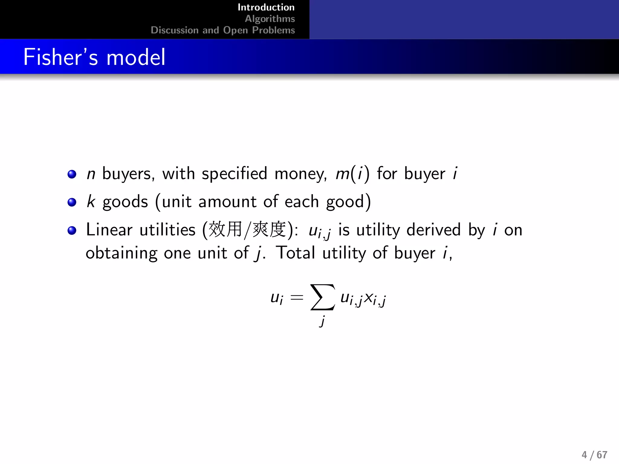
Combinatorial Algorithm for Fisher’s Model
No LP’s known for capturing equilibrium
allocations for Fisher’s model, although this
model doesn’t require integer constraints.
max
i
ui , s.t.,
j
pj xi,j ≤ mi , ui =
j
ui,jxi,j
Devanur, Papadimitriou, Saberi, and Vazirani,
2002[1]
Use primal-dual schema. It is highly successful algorithm
design technique from exact and approximation algorithms
11 / 67](https://image.slidesharecdn.com/slides-090326043049-phpapp01-150607173359-lva1-app6891/75/Introduction-to-Algorithmic-aspect-of-Market-Equlibra-11-2048.jpg)
![Introduction
Algorithms
Discussion and Open Problems
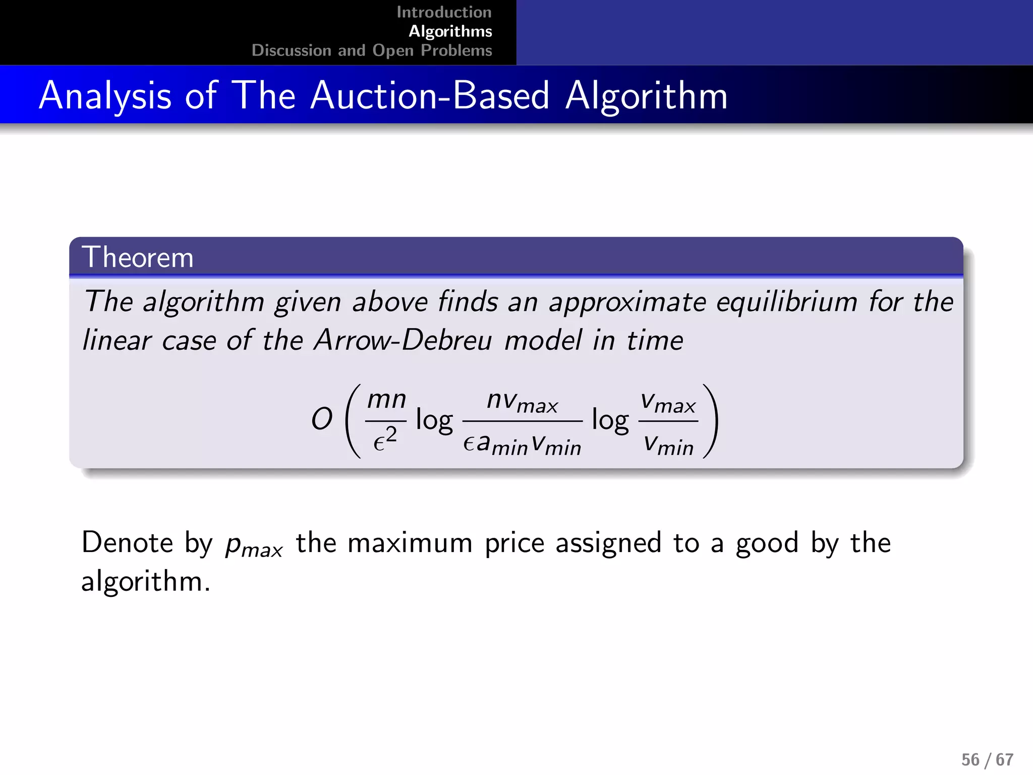
Arrow-Debreu model: An Auction-Based Algorithm
Jain proved that Arrow-Debreu’s Model with Linear Utility
Functions is in P at 2007[4], however it is based on ellipsoid
algorithm. And ellipsoid algorithm is slow in practice.
Garg et al. [3] proposed an auction-based PTAS for the linear
case of the Arrow-Debreu model.
52 / 67](https://image.slidesharecdn.com/slides-090326043049-phpapp01-150607173359-lva1-app6891/75/Introduction-to-Algorithmic-aspect-of-Market-Equlibra-52-2048.jpg)
![Introduction
Algorithms
Discussion and Open Problems
An Auction-Based Algorithm[3]
1 Initializes the price of each good to be unit, computes the
worth of the initial endowment of each agent, and gives this
money to each agent. All goods are initially fully unsold.
2 LOOP UNTIL (the surplus of the traders becomes sufficiently
small, i.e., amin, or all the goods are assigned.)1
2.1 LOOP UNTIL (no agent has surplus money)
2.1.1 Agent i outbid to buy her optimal good j as many as possible,
i.e., at price (1 + )pj .
2.1.2 If agent i has all good j, update the worth of agents with
price (1 + )pj . And Jump to [2].
1
amin means the minimum amount of initial endowments which a agent has.
53 / 67](https://image.slidesharecdn.com/slides-090326043049-phpapp01-150607173359-lva1-app6891/75/Introduction-to-Algorithmic-aspect-of-Market-Equlibra-53-2048.jpg)

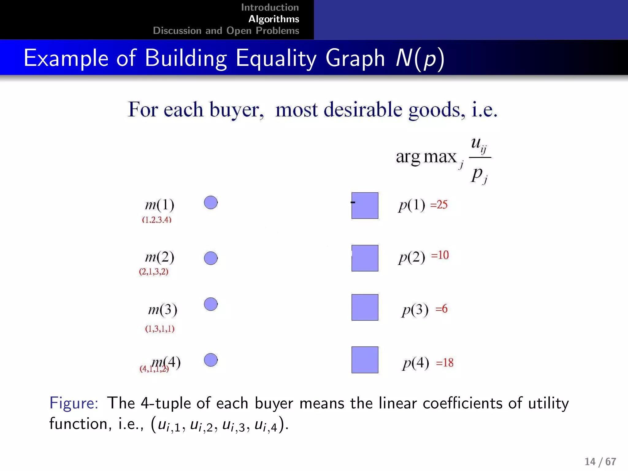
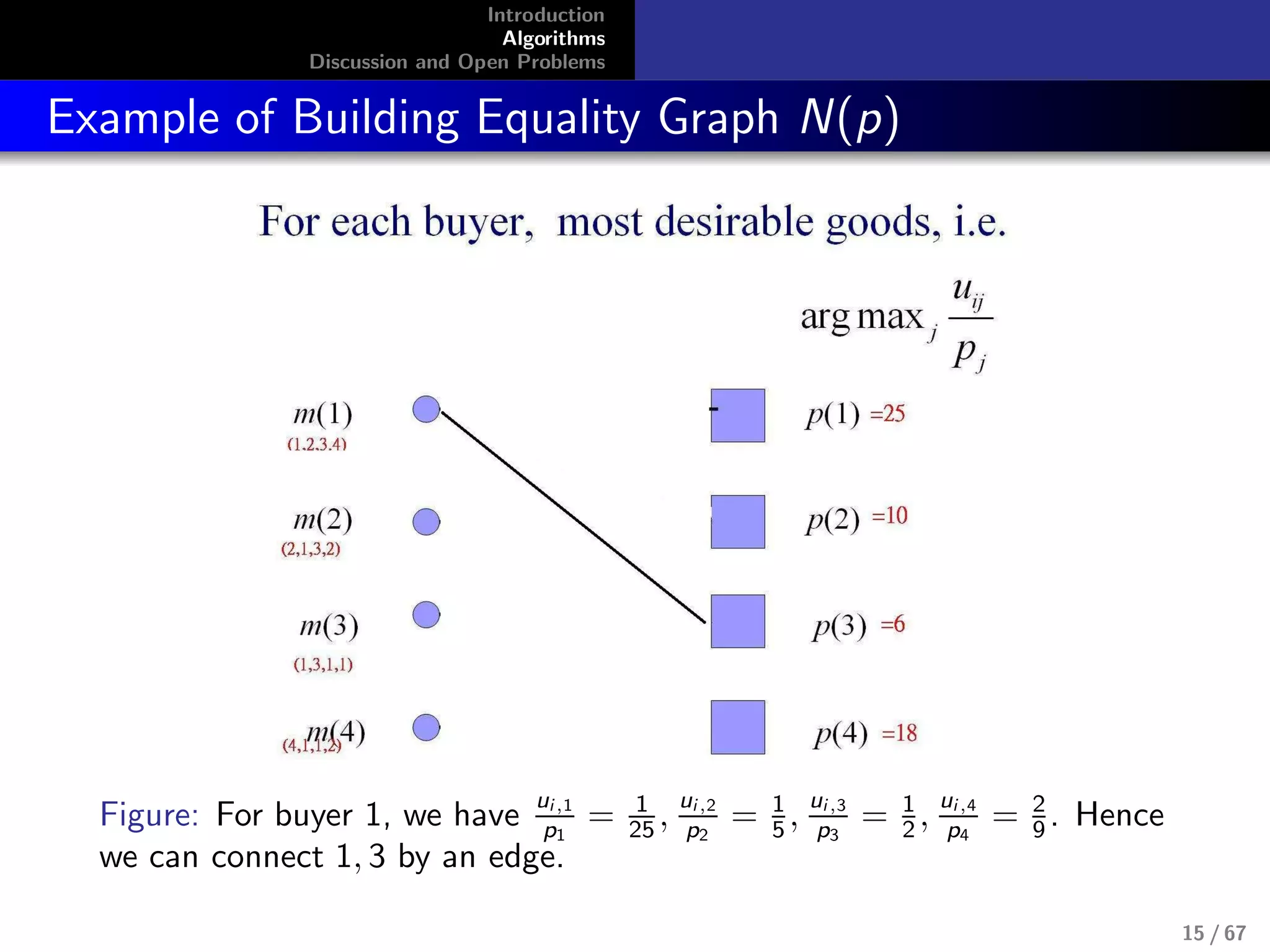
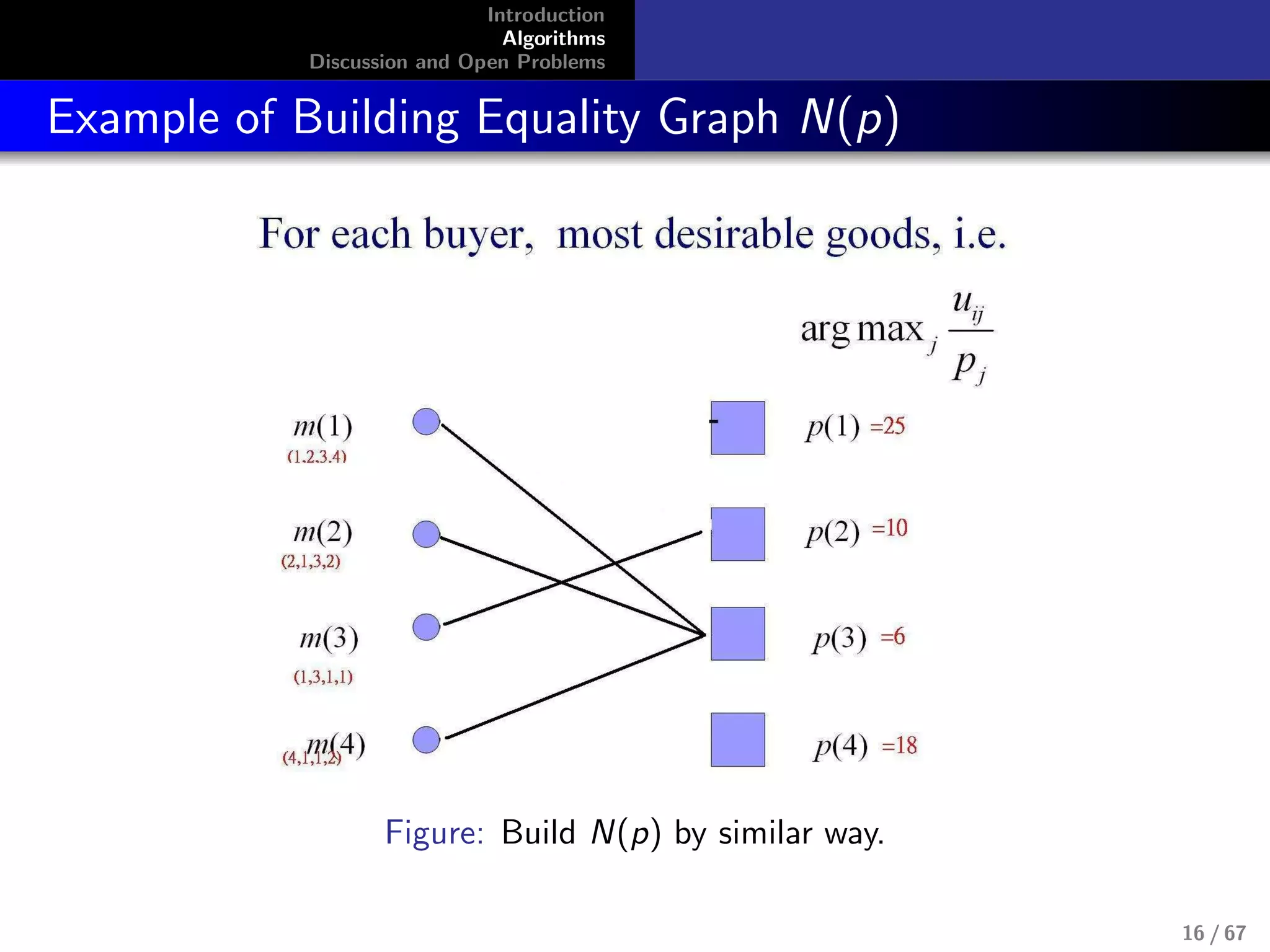
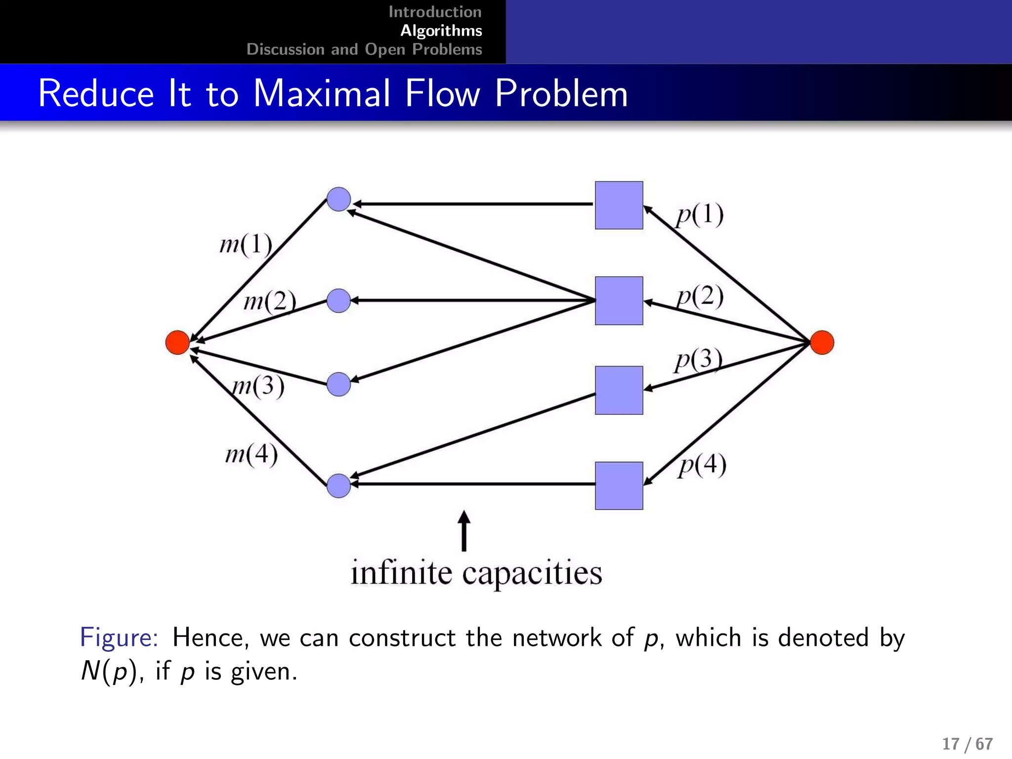
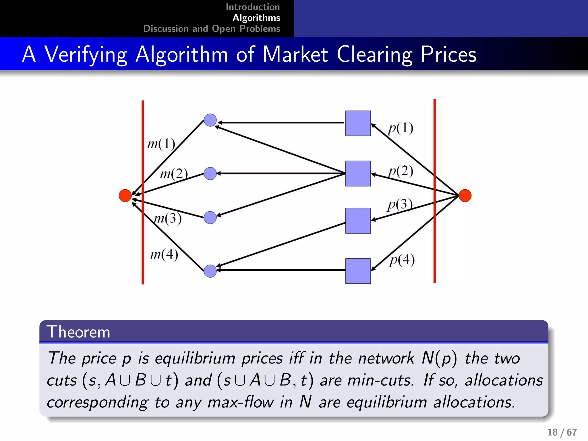
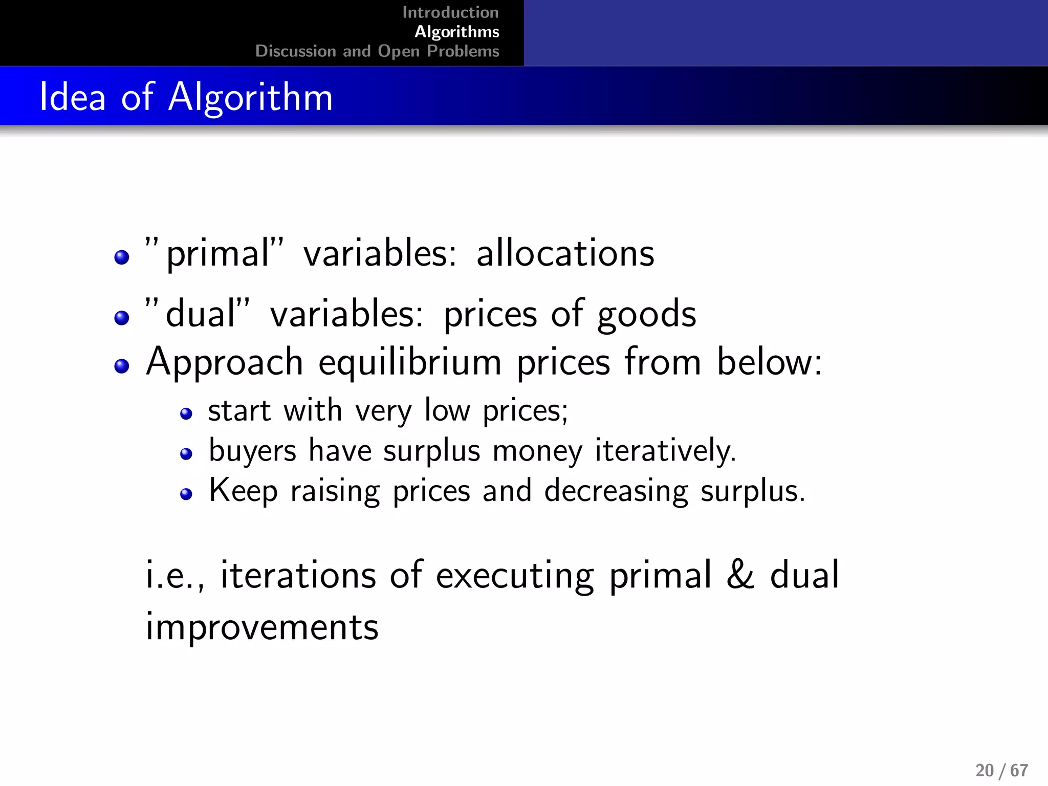
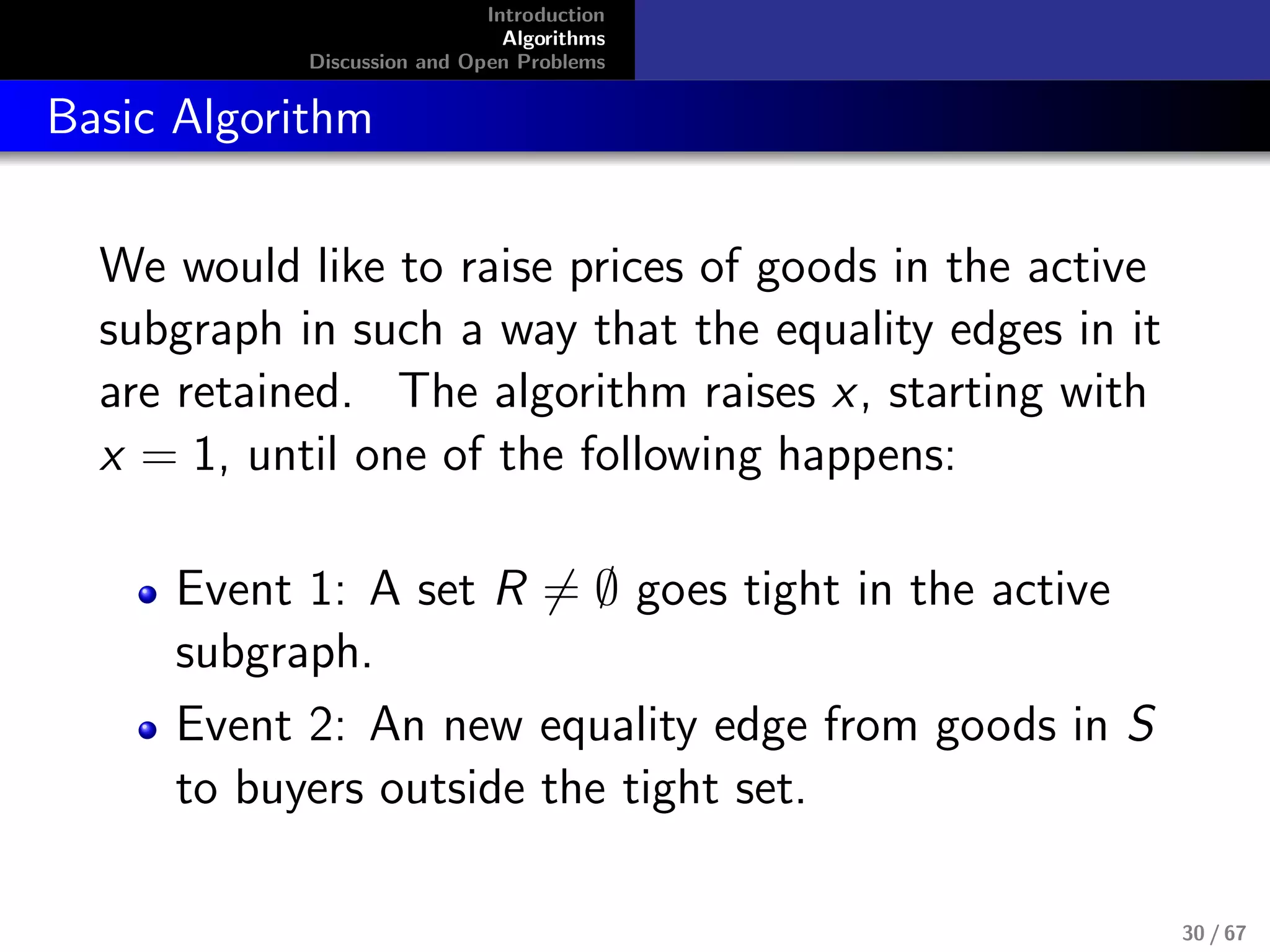
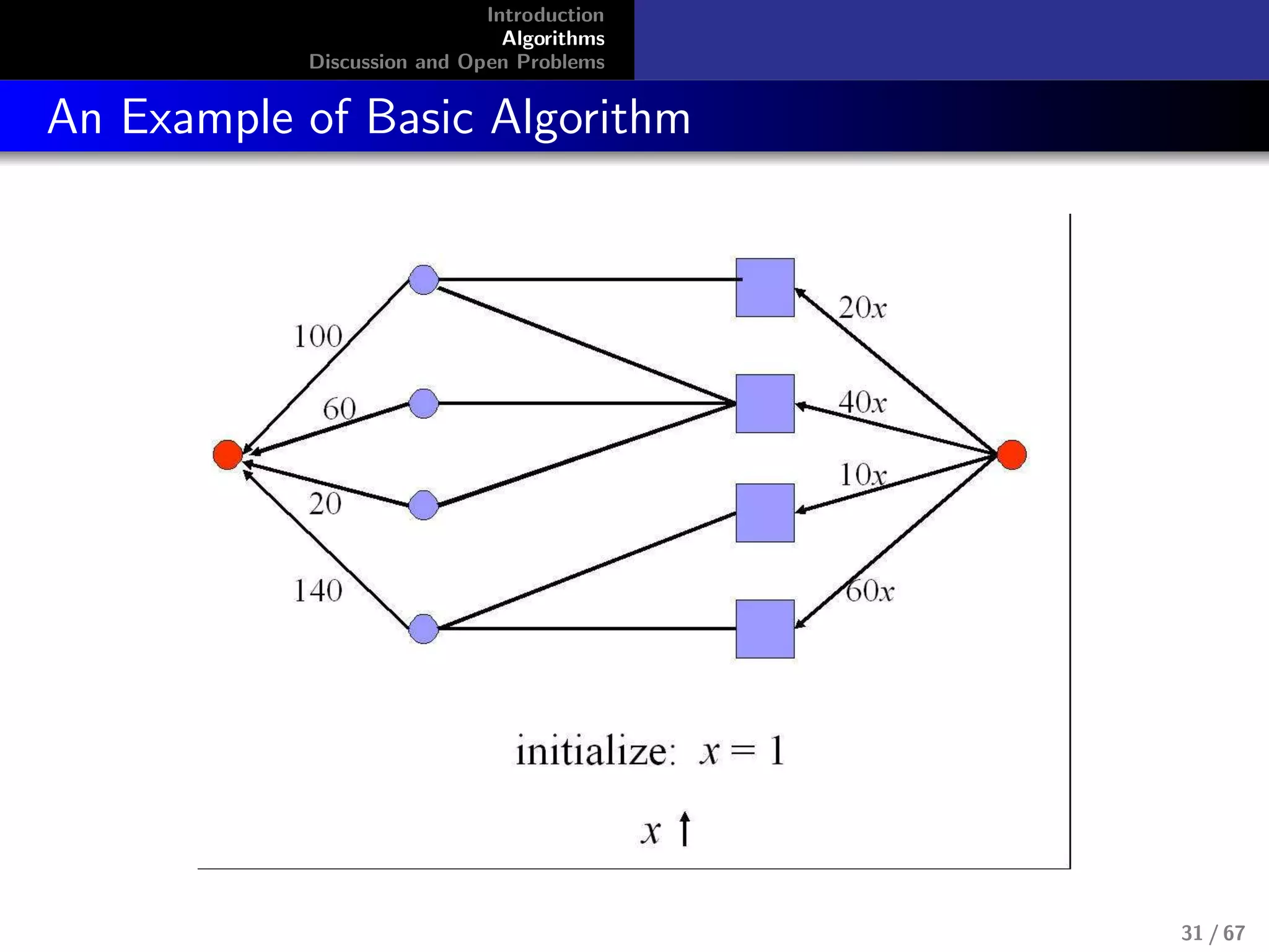
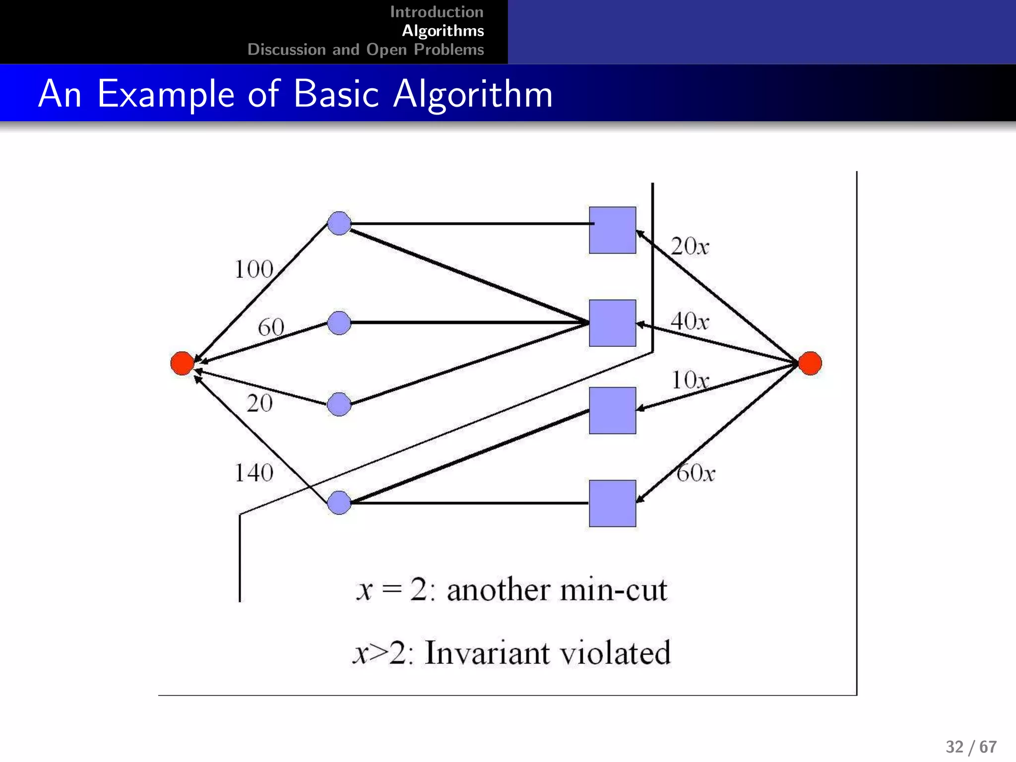
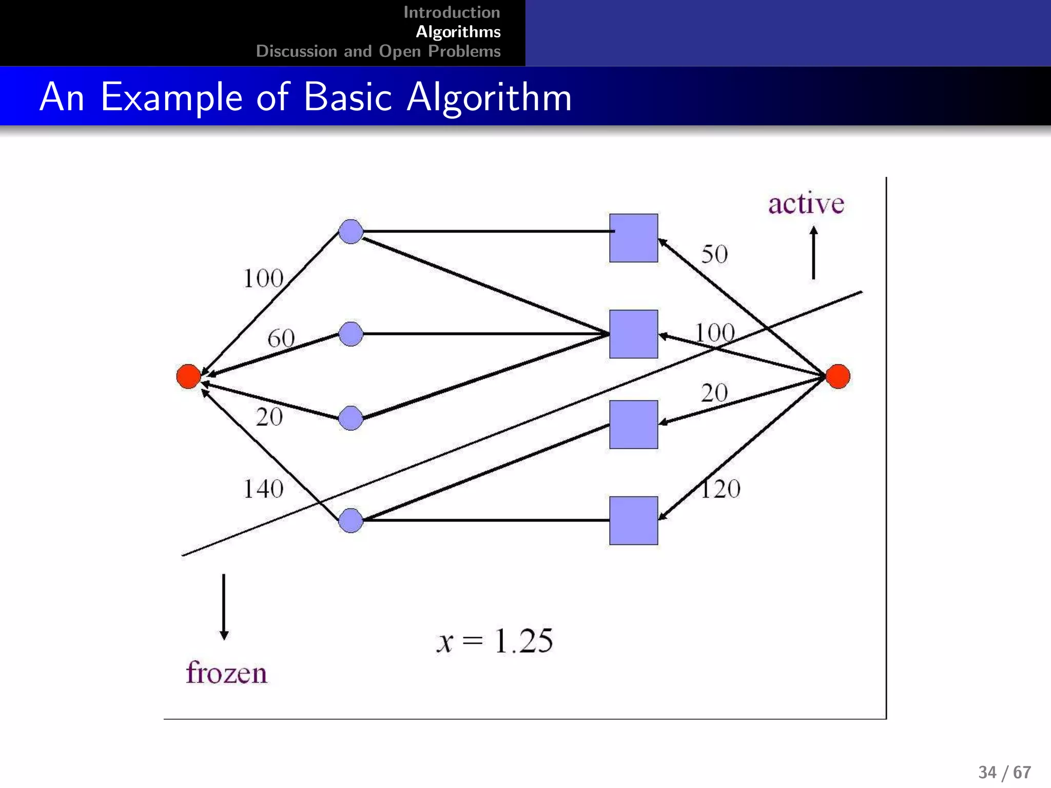
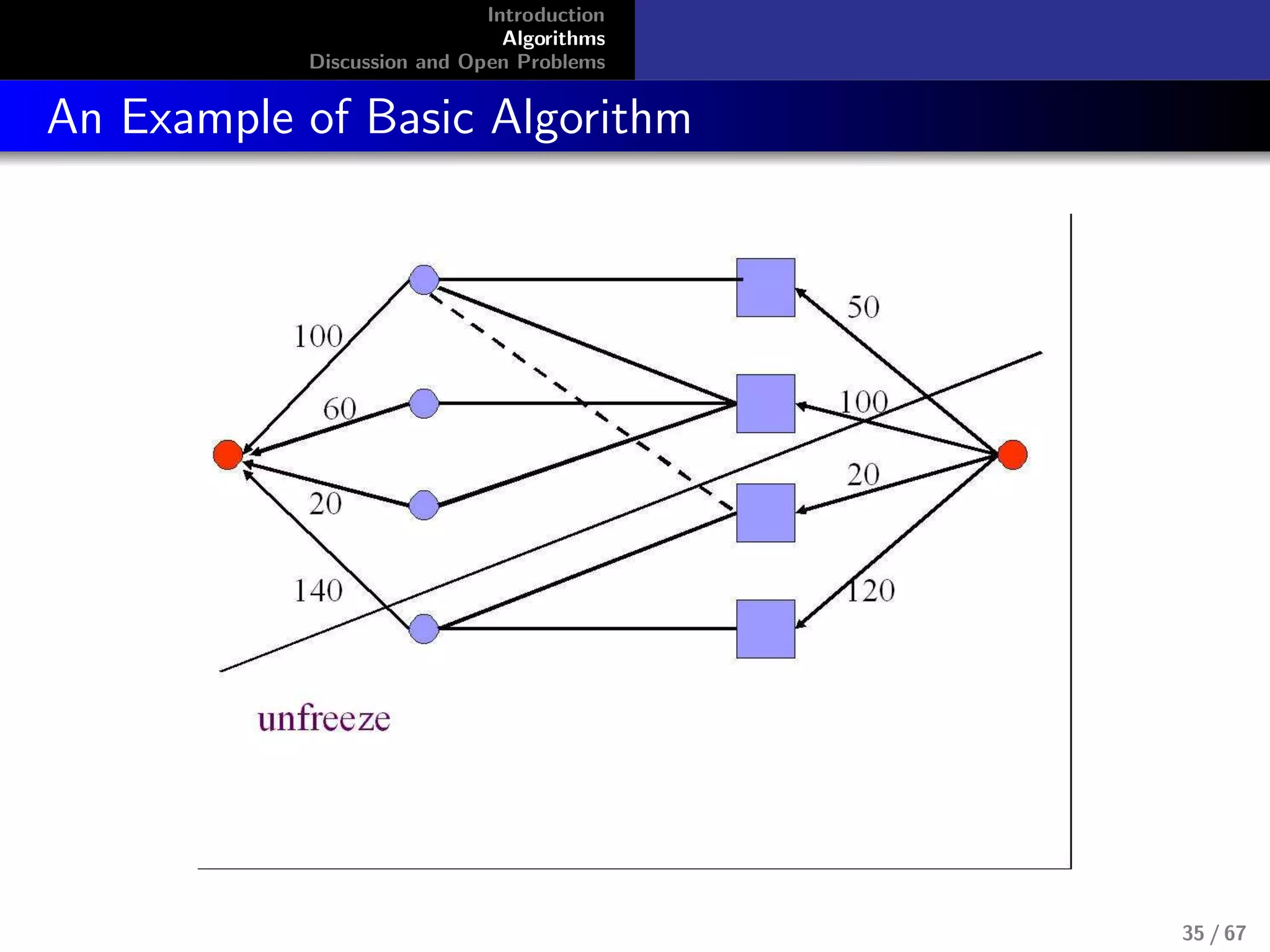
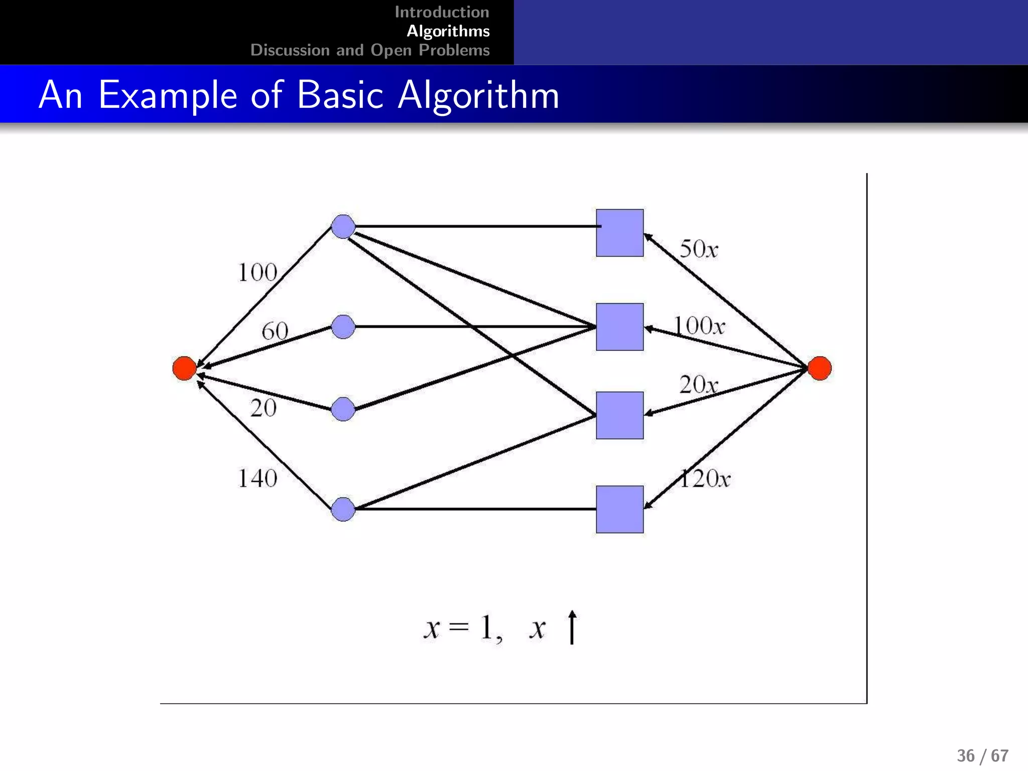
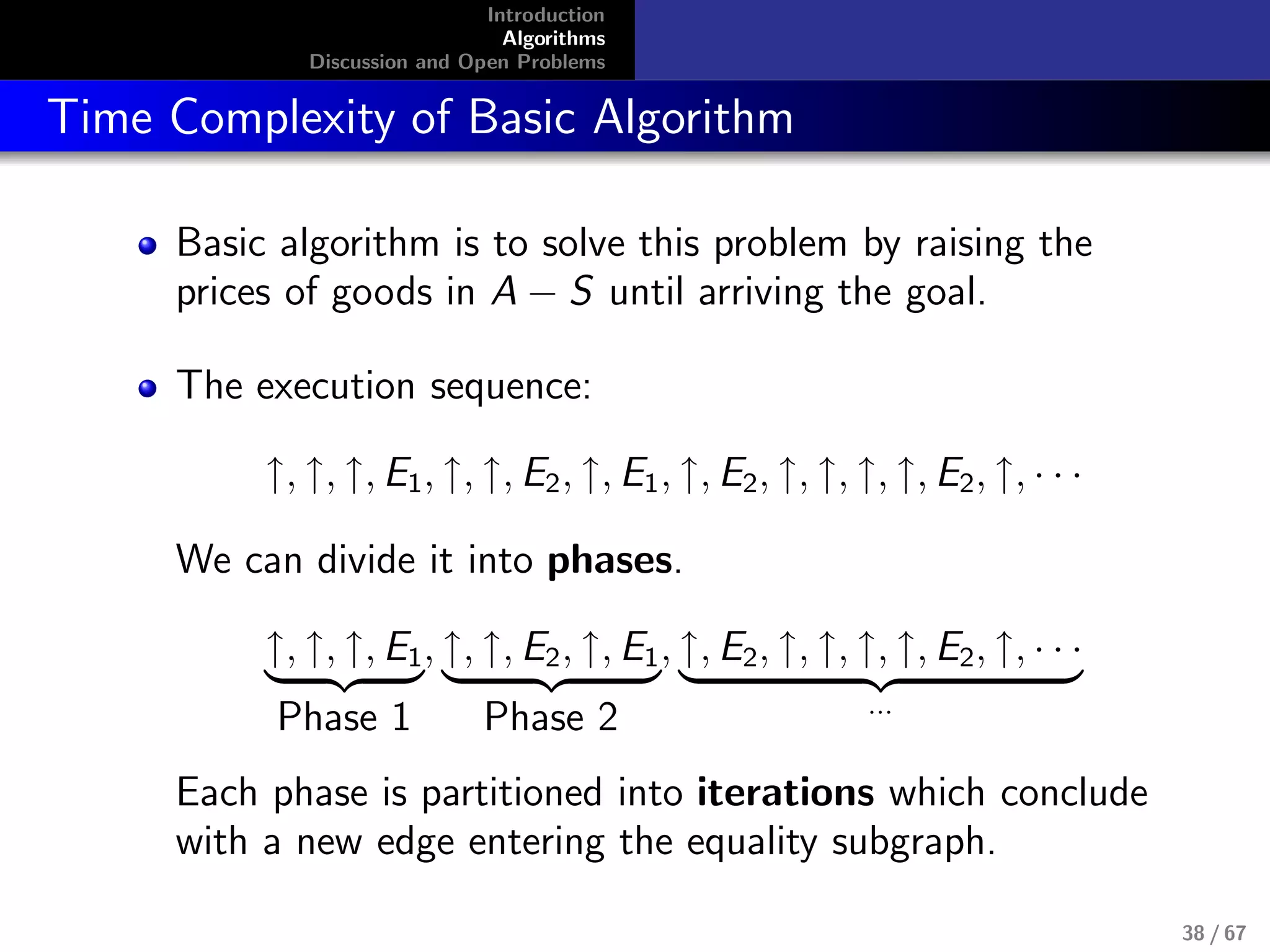
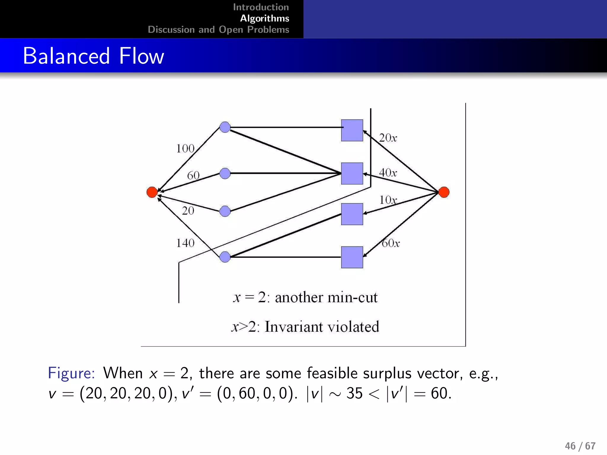
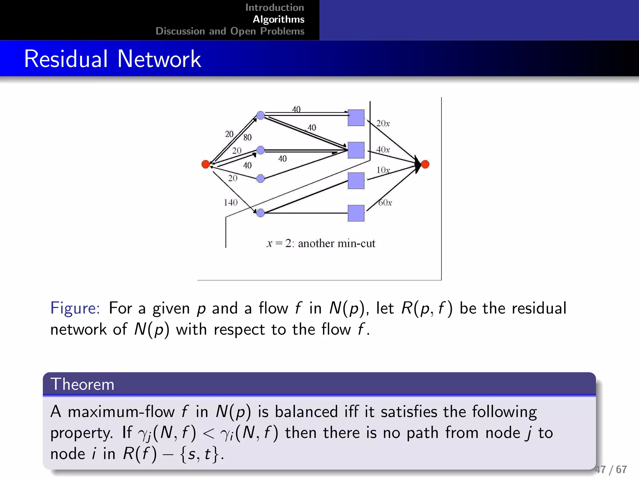
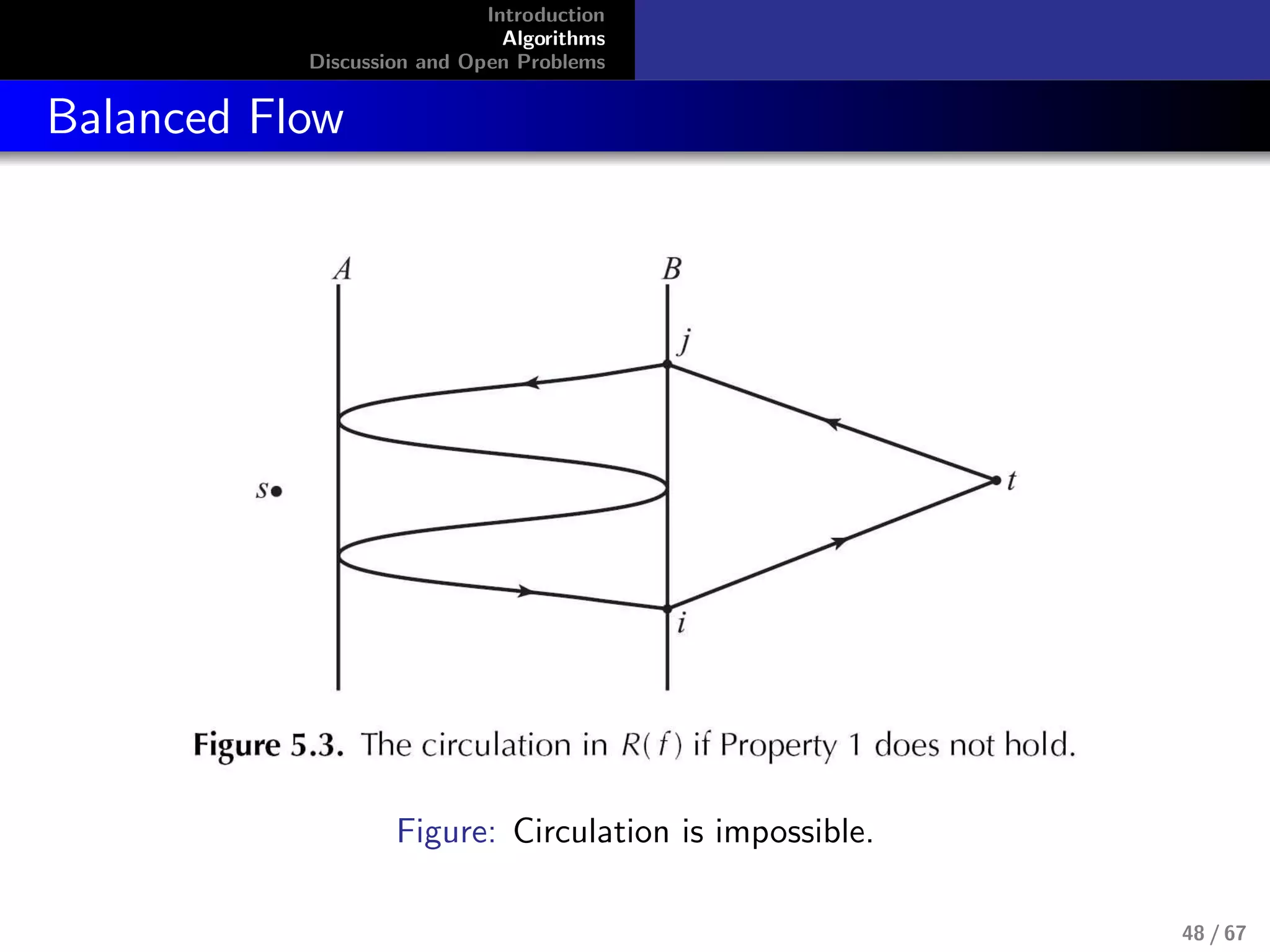
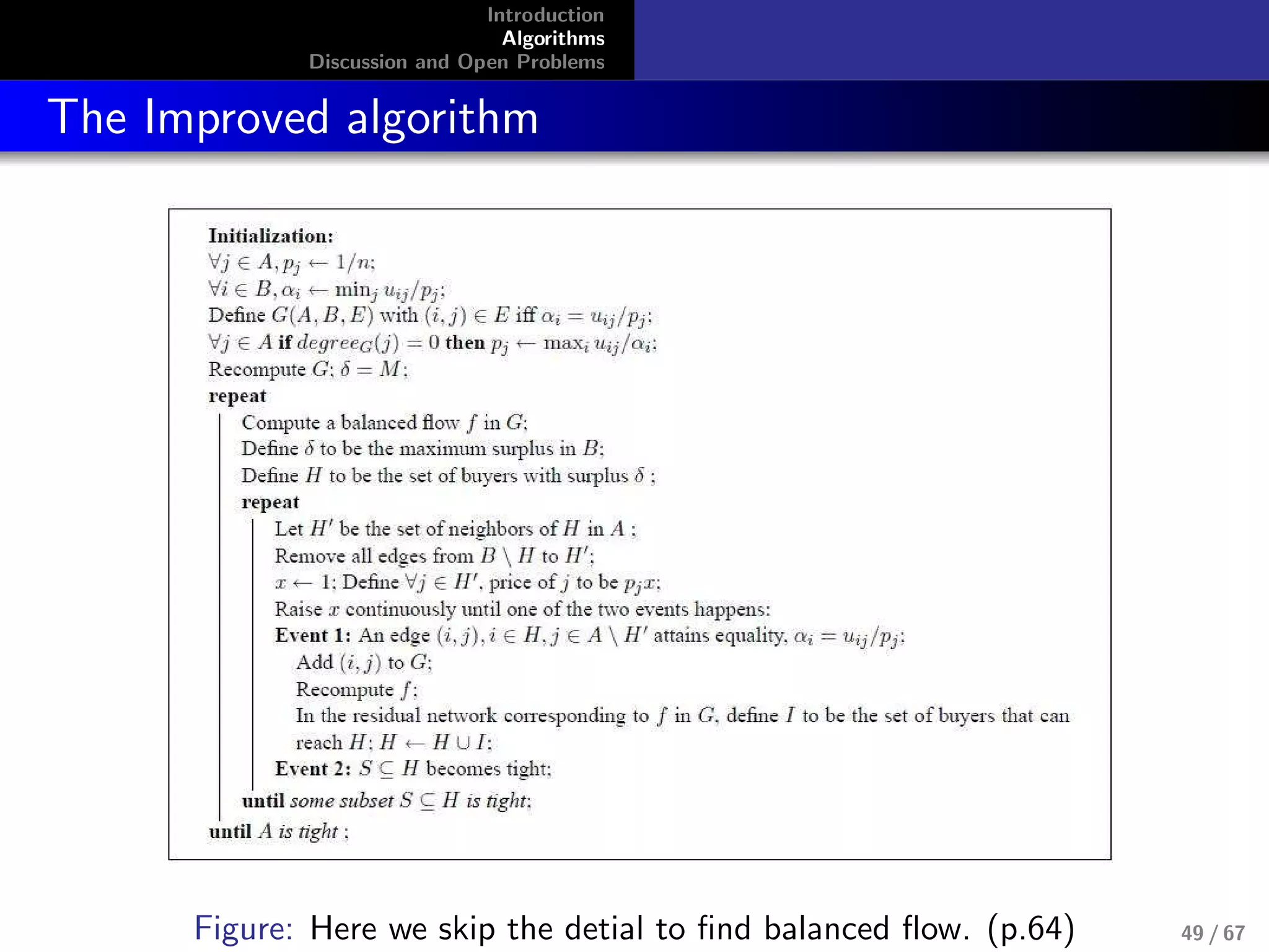
The document discusses algorithms for computing market equilibria in economic models. It introduces Fisher's model and the Arrow-Debreu model of markets. It describes how competitive equilibria and Pareto efficiency arise in these models under certain assumptions. The document then presents an algorithm based on a primal-dual approach that computes market clearing prices for Fisher's linear model in polynomial time by incrementally raising prices until surplus is eliminated.