The document provides an introduction to Probabilistic Latent Semantic Analysis (PLSA). It discusses how PLSA improves on previous Latent Semantic Analysis methods by incorporating a probabilistic framework. PLSA models documents as mixtures of topics and allows words to have multiple meanings. The parameters of the PLSA model, including the topic distributions and word-topic distributions, are estimated using an expectation-maximization algorithm to find the parameters that best explain the observed word-document co-occurrence data.

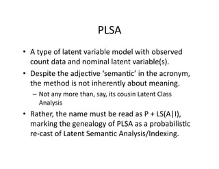
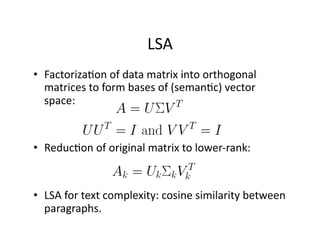
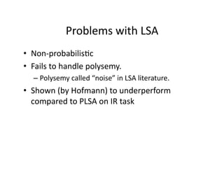
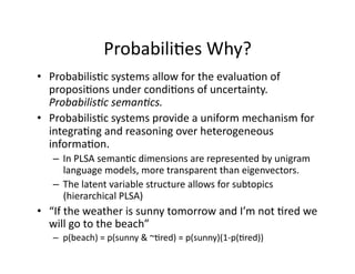
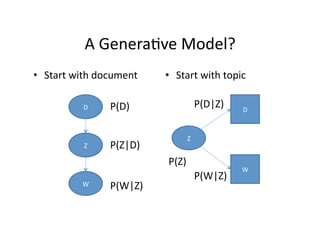
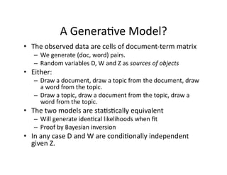
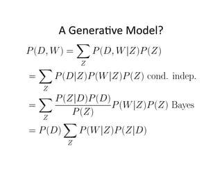
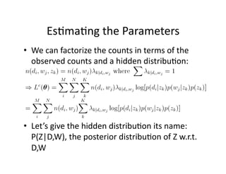
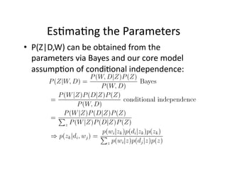
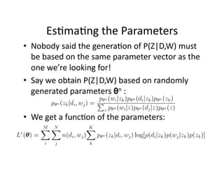
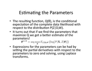
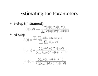
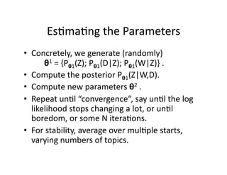
1. Introduc)on to Probabilis)c
Latent Seman)c Analysis
NYP Predic)ve Analy)cs Meetup
June 10, 2010

2. PLSA
• A type of latent variable model with observed
count data and nominal latent variable(s).
• Despite the adjec)ve ‘seman)c’ in the acronym,
the method is not inherently about meaning.
– Not any more than, say, its cousin Latent Class
Analysis
• Rather, the name must be read as P + LS(A|I),
marking the genealogy of PLSA as a probabilis)c
re‐cast of Latent Seman)c Analysis/Indexing.

3. LSA
• Factoriza)on of data matrix into orthogonal
matrices to form bases of (seman)c) vector
space:
• Reduc)on of original matrix to lower‐rank:
• LSA for text complexity: cosine similarity between
paragraphs.

4. Problems with LSA
• Non‐probabilis)c
• Fails to handle polysemy.
– Polysemy called “noise” in LSA literature.
• Shown (by Hofmann) to underperform
compared to PLSA on IR task

5. Probabili)es Why?
• Probabilis)c systems allow for the evalua)on of
proposi)ons under condi)ons of uncertainty.
Probabilis)c seman)cs.
• Probabilis)c systems provide a uniform mechanism for
integra)ng and reasoning over heterogeneous
informa)on.
– In PLSA seman)c dimensions are represented by unigram
language models, more transparent than eigenvectors.
– The latent variable structure allows for subtopics
(hierarchical PLSA)
• “If the weather is sunny tomorrow and I’m not )red we
will go to the beach”
– p(beach) = p(sunny & ~)red) = p(sunny)(1‐p()red))

6. A Genera)ve Model?
• Let X be a random vector with components {X1,
X2, … , Xn} random variables.
• Each realiza)on of X is assigned to a class, one of
a random variable Y.
• A genera(ve model tells a story about how the
Xs came about: “once upon a )me, a Y was
selected, then Xs were created out of that Y”.
• A discrimina(ve model strives to iden)fy, as
unambiguously as possible, the Y value for some
given X

7. A Genera)ve Model?
• A discrimina)ve model es)mates P(Y|X)
directly.
• A genera)ve model es)mates P(X|Y) and P(Y)
– The predic)ve direc)on is then computed via
Bayesian inversion:
where P(X) is obtained by condi)oning on Y:

8. A Genera)ve Model?
• A classic genera)ve/discrimina)ve pair: Naïve
Bayes vs Logis)c Regression.
• Naïve Bayes assumes that the Xis are
condi)onally independent given Y, so it es)mates
P(Xi | Y).
• Logis)c regression makes other assump)ons, e.g.
linearity of the independent variables with logit
of dependent, independence of errors, but
handles correlated predictors (up to perfect
collinearity).

9. A Genera)ve Model?
• Genera)ve models have richer probabilis)c
seman)cs.
– Func)ons run both way.
– Assign distribu)ons to the “independent” variables,
even previously unseen realiza)ons.
• Ng and Jordan (2002) show that logis)c
regression has higher asympto)c accuracy, but
converges more slowly, sugges)ng a trade‐off
between accuracy and variance.
• Overall trade‐off between accuracy and
usefulness.

10. A Genera)ve Model?
• Start with document • Start with topic
D P(D) P(D|Z) D
Z
Z P(Z|D)
P(Z)
W
P(W|Z)
W P(W|Z)

11. A Genera)ve Model?
• The observed data are cells of document‐term matrix
– We generate (doc, word) pairs.
– Random variables D, W and Z as sources of objects
• Either:
– Draw a document, draw a topic from the document, draw
a word from the topic.
– Draw a topic, draw a document from the topic, draw a
word from the topic.
• The two models are sta)s)cally equivalent
– Will generate iden)cal likelihoods when fit
– Proof by Bayesian inversion
• In any case D and W are condi)onally independent
given Z.

12. A Genera)ve Model?

13. A Genera)ve Model?
• But what is a Document here?
– Just a label! There are no anributes associated with
documents.
– P(D|Z) relates topics to labels
• A previously unseen document is just a new label
• Therefore PLSA isn’t genera)ve in an interes)ng
way, as it cannot handle previously unseen inputs
in a genera)ve manner.
– Though the P(Z) distribu)on may s)ll be of interest.

14. Es)ma)ng the Parameters
• Θ = {P(Z); P(D|Z); P(W|Z)}
• All distribu)ons refer to latent variable Z, so
cannot be es)mated directly from the data.
• How do we know when we have the right
parameters?
– When we have the θ that most closely generates
the data, i.e. the document‐term matrix

15. Es)ma)ng the Parameters
• The joint P(D,W) generates the observed
document‐term matrix.
• The parameter vector θ yields the joint P(D,W)
• We want θ that maximizes the probability of
the observed data.

16. Es)ma)ng the Parameters
• For the mul)nomial distribu)on,
• Let X be the MxN document‐term matrix.

17. Es)ma)ng the Parameters
• Imagine we knew the X’ = MxNxK complete
data matrix, where the counts for topics were
overt. Then,
New and interes)ng: The usual parameters θ
unseen counts must sum
to 1 for given d,w

18. Es)ma)ng the Parameters
• We can factorize the counts in terms of the
observed counts and a hidden distribu)on:
• Let’s give the hidden distribu)on its name:
P(Z|D,W), the posterior distribu)on of Z w.r.t.
D,W

19. Es)ma)ng the Parameters
• P(Z|D,W) can be obtained from the
parameters via Bayes and our core model
assump)on of condi)onal independence:

20. Es)ma)ng the Parameters
• Nobody said the genera)on of P(Z|D,W) must
be based on the same parameter vector as the
one we’re looking for!
• Say we obtain P(Z|D,W) based on randomly
generated parameters θn :
• We get a func)on of the parameters:

21. Es)ma)ng the Parameters
• The resul)ng func)on, Q(θ), is the condi)onal
expecta)on of the complete data likelihood with
respect to the distribu)on P(Z|D,W).
• It turns out that if we find the parameters that
maximize Q we get a bener es)mate of the
parameters!
• Expressions for the parameters can be had by
sesng the par)al deriva)ves with respect to the
parameters to zero and solving, using Laplace
transforms.

22. Es)ma)ng the Parameters
• E‐step (misnamed)
• M‐step

23. Es)ma)ng the Parameters
• Concretely, we generate (randomly)
θ1 = {Pθ1(Z); Pθ1(D|Z); Pθ1(W|Z)} .
• Compute the posterior Pθ1(Z|W,D).
• Compute new parameters θ2 .
• Repeat un)l “convergence”, say un)l the log
likelihood stops changing a lot, or un)l
boredom, or some N itera)ons.
• For stability, average over mul)ple starts,
varying numbers of topics.

24. Folding In
• When a new document comes along, we want to
es)mate the posterior of the topics for the
document.
– What is it about? I.e. what is the distribu)on over
topics of the new document?
• Perform a “linle EM”:
– E‐step: compute P(Z|W, Dnew)
– M‐step: compute P(Z|Dnew) keeping all other
parameters unchanged.
– Converges very fast, five itera)ons?
– Overtly discrimina)ve! The true colors of the method
emerge.

25. Problems with PLSA
• Easily huge number of parameters
– Leads to unstable es)ma)on (local maxima).
– Computa)onally intractable because of huge
matrices
– Modeling the documents directly can be problem
• What if the collec)on has millions of documents?
• Not properly genera)ve (is this a problem?)

26. Examples of Applica)ons
• Informa)on Retrieval: compare topic
distribu)ons for documents and queries using
a similarity measure like rela)ve entropy.
• Collabora)ve Filtering (Hoffman, 2002) using
Gaussian PLSA.
• Topic segmenta)on in texts, by looking for
spikes in the distances between topic
distribu)ons for neighbouring text blocks.