CS 446:  Machine Learning Gerald DeJong [email_address] 3-0491 3320 SC Recent approval for a TA to be named later
Office hours: after most classes and Thur @ 3 Text: Mitchell’s Machine Learning Midterm: Oct. 4 Final: Dec. 12 each a third Homeworks / projects Submit at the beginning of class Late penalty: 20% / day up to 3 days Programming, some in-class assignments Class web site soon Cheating: none allowed!  We adopt dept. policy
Please answer these and hand in now Name Department Where (If?*) you had Intro AI course Who taught it (esp. if not here) 1) Why interested in Machine Learning? 2) Any topics you would like to see covered? * may require significant additional effort
Approx. Course Overview / Topics Introduction:  Basic problems and questions   A detailed examples:  Linear threshold units Basic Paradigms: PAC (Risk Minimization); Bayesian Theory; SRM (Structural Risk Minimization); Compression; Maximum Entropy;… Generative/Discriminative; Classification/Skill;… Learning Protocols Online/Batch;  Supervised/Unsupervised/Semi-supervised; Delayed supervision Algorithms:  Decision Trees (C4.5) [Rules and ILP (Ripper, Foil)] Linear Threshold Units (Winnow, Perceptron; Boosting; SVMs; Kernels) Probabilistic Representations (naïve Bayes, Bayesian trees; density estimation) Delayed supervision: RL Unsupervised/Semi-supervised: EM Clustering, Dimensionality Reduction, or others of student interest
What to Learn Classifiers:   Learn a hidden function   Concept Learning:  chair ?  face ?  game ? Diagnosis:  medical; risk assessment Models:   Learn a map  (and use it to navigate) Learn a distribution  (and use it to answer queries) Learn a language model;  Learn an Automaton Skills: Learn to play games; Learn a Plan / Policy Learn to Reason; Learn to Plan Clusterings:  Shapes of objects; Functionality; Segmentation Abstraction Focus on  classification   (importance, theoretical richness, generality,…)
What to Learn?  Direct Learning: (discriminative, model-free[bad name]) Learn a function that maps an input instance to the sought after property. Model Learning: (indirect, generative) Learning a model of the domain; then use it to answer various questions about the domain In both cases, several protocols can be used –  Supervised – learner is given examples and answers Unsupervised – examples, but no answers Semi-supervised – some examples w/answers, others w/o Delayed supervision
Supervised  Learning Given:   Examples  (x,f  ( x))   of some unknown function   f   Find:  A good approximation to  f   x  provides some representation of the input The process of mapping a domain element into a representation is called  Feature Extraction. (Hard; ill-understood; important) x   2  {0,1} n   or  x   2   < n   The target function (label)  f(x)   2  {-1,+1}  Binary Classification  f(x)   2  {1,2,3,.,k-1}  Multi-class classification  f(x)   2   <    Regression
Example and Hypothesis Spaces X H X: Example Space – set of all well-formed inputs [w/a distribution] H: Hypothesis Space – set of all well-formed outputs - - + + + - - - +
Supervised  Learning: Examples Disease diagnosis  x: Properties of patient (symptoms, lab tests) f : Disease (or maybe: recommended therapy) Part-of-Speech tagging  x: An English sentence (e.g., The  can  will rust) f : The part of speech of a word in the sentence Face recognition  x: Bitmap picture of person’s face f : Name the person (or maybe: a property of) Automatic Steering x: Bitmap picture of road surface in front of car f : Degrees to turn the steering wheel
y  =  f  (x 1 , x 2 , x 3 , x 4 ) Unknown function x 1 x 2 x 3 x 4 A  Learning Problem X H ? ? (Boolean: x1, x2, x3, x4,  f )
y  =  f  (x 1 , x 2 , x 3 , x 4 ) Unknown function x 1 x 2 x 3 x 4 Training Set Example  x 1   x 2   x 3   x 4  y 1   0  0  1  0  0 3   0  0  1  1  1 4  1  0  0  1  1 5   0  1  1  0  0 6  1  1  0  0  0 7  0  1  0  1  0 2   0  1  0  0  0
Hypothesis Space Complete Ignorance:  How many possible functions? 2 16   = 56536 over four input features.   After seven examples how many possibilities for f? 2 9   possibilities remain for   f How many examples until we figure out which is correct? We need to see labels for all 16 examples! Is Learning Possible?   Example  x 1   x 2   x 3   x 4  y 1  1  1  1  ? 0  0  0  0  ? 1  0  0  0  ? 1  0  1  1  ? 1  1  0  0  0 1  1  0  1  ? 1  0  1  0  ? 1  0  0  1  1 0  1  0  0  0 0  1  0  1  0 0  1  1  0  0 0  1  1  1  ? 0  0  1  1  1 0  0  1  0  0 0  0  0  1  ? 1  1  1  0  ?
Another Hypothesis Space Simple Rules:  There are  only 16 simple   conjunctive rules of the form  y=x i   Æ  x j   Æ  x k ... No simple rule explains the data. The same is true for simple clauses 1   0  0  1  0  0 3   0  0  1  1  1 4  1  0  0  1  1 5   0  1  1  0  0 6  1  1  0  0  0 7  0  1  0  1  0 2   0  1  0  0  0 y =c  x 1  1100  0 x 2  0100  0 x 3  0110  0 x 4  0101  1 x 1     x 2   1100  0 x 1     x 3  0011  1 x 1     x 4  0011  1 Rule  Counterexample x 2     x 3  0011  1 x 2     x 4  0011  1 x 3     x 4  1001  1 x 1     x 2     x 3  0011 1 x 1     x 2     x 4  0011 1 x 1     x 3     x 4  0011 1 x 2     x 3     x 4  0011 1 x 1     x 2     x 3     x 4  0011 1 Rule  Counterexample
Third Hypothesis Space m-of-n rules:  There are 29 possible rules  of the form  ”y = 1  if and only if at least  m  of the following  n  variables are  1” Found a consistent hypothesis. 1   0  0  1  0  0 3   0  0  1  1  1 4  1  0  0  1  1 5   0  1  1  0  0 6  1  1  0  0  0 7  0  1  0  1  0 2   0  1  0  0  0  x 1    3  -  -  -  x 2    2  -  -  -  x 3    1  -  -  -  x 4    7  -  -  -  x 1, x 2    2  3  -  -  x 1,  x 3    1  3  -  -  x 1,  x 4    6  3  -  -  x 2, x 3    2  3  -  - variables  1 -of  2 -of  3 -of  4 -of  x 2,  x 4    2  3  -  -   x 3,  x 4    4  4  -  -  x 1, x 2,  x 3    1  3  3  -  x 1, x 2,  x 4    2  3  3  -  x 1, x 3, x 4    1           3  -  x 2,  x 3, x 4    1  5  3  -  x 1,  x 2,  x 3, x 4    1  5  3  3 variables  1 -of  2 -of  3 -of  4 -of
Views of Learning Learning is the removal of our remaining uncertainty:  Suppose we  knew  that the unknown function was an m-of-n Boolean function, then we could use the training data to infer which function it is. Learning requires guessing a good, small hypothesis class :  We can start with a very small class and enlarge it until it contains an hypothesis that fits the data. We could be wrong ! Our prior knowledge might be wrong:  y=x4    one-of (x1, x3) is also consistent   Our guess of the hypothesis class could be wrong   If this is the unknown function, then we will make errors when we are given new  examples, and are asked to predict the value of the function
General strategy for Machine Learning   H should respect our prior understanding:  Excess expressivity makes learning difficult Expressivity of H should match our ignorance Understand flexibility of std. hypothesis spaces:  Decision trees, neural networks, rule grammars, stochastic models Hypothesis spaces of flexible size;   Nested collections of hypotheses.  ML succeeds when these interrelate Develop algorithms for finding a hypothesis h that fits the data  h will likely perform well when the richness of H is less than the information in the training set
Terminology Training example:  An pair of the form (x, f (x))  Target function (concept):  The true function f (?) Hypothesis:  A proposed function h, believed to be similar to f.  Concept:  Boolean function.  Example for which f (x)= 1 are  positive  examples; those for which  f (x)= 0 are  negative  examples (instances)  (sometimes used interchangeably w/ “Hypothesis”) Classifier:  A discrete valued function. The possible value of f: {1,2,…K} are the classes or  class labels .  Hypothesis space:  The space of all hypotheses that can, in principle, be output by the learning algorithm. Version Space:  The space of all hypothesis in the hypothesis space that have not yet been ruled out.
Key Issues in Machine Learning Modeling How to formulate application problems as machine learning problems ? Learning Protocols (where is the data coming from, how?)  Project examples:  [complete products] EMAIL Given a seminar announcement, place the relevant information in my outlook Given a message, place it in the appropriate folder Image processing:  Given a folder with pictures; automatically rotate all those that need it. My office:  have my office greet me in the morning and unlock the door (but do it only for me!)  Context Sensitive Spelling:  Incorporate into Word
Key Issues in Machine Learning Modeling How to formulate application problems as machine learning problems ? Learning Protocols (where is the data coming from, how?)  Representation:  What are good hypothesis spaces ?  Any rigorous way to find these? Any general approach? Algorithms:  What are good algorithms?  How do we define success?  Generalization Vs. over fitting The computational problem
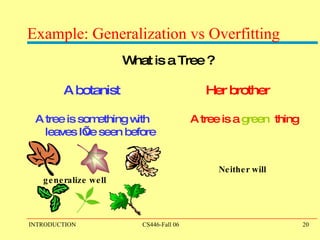
Example: Generalization vs Overfitting What is a Tree ? A botanist   Her brother   A tree is something with   A tree is a  green   thing   leaves I’ve seen before   Neither will generalize well
Self-organize into Groups of 4 or 5 Assignment 1 The Badges Game …… Prediction or Modeling? Representation Background Knowledge When did learning take place? Learning Protocol? What is the problem? Algorithms
Linear Discriminators I don’t know { whether,   weather}   to laugh or cry How can we make this a learning problem? We will look for a function  F: Sentences   { whether,   weather}   We need to define the domain of this function better. An option : For each word  w  in English define a  Boolean  feature x w  :  [x w  =1] iff w is in the sentence This maps a sentence to a point in {0,1} 50,000 In this space:  some points are  whether   points some are  weather   points Learning Protocol? Supervised? Unsupervised?
What’s Good?  Learning problem :  Find a function that  best separates the data What function? What’s best? How to find it? A possibility: Define the learning problem to be: Find a (linear) function that best separates the data
Exclusive-OR  (XOR) (x 1   Æ  x 2)   Ç  ( : {x 1 }  Æ   : {x 2 }) In general: a parity function. x i   2  {0,1} f(x 1 , x 2 ,…, x n ) = 1  iff    x i  is even This function is not  linearly separable . x 1 x 2
Sometimes Functions Can be Made Linear x 1  x 2  x 4   Ç  x 2  x 4  x 5   Ç  x 1  x 3  x 7 Space: X= x 1 , x 2 ,…, x n input Transformation New Space: Y = {y 1 ,y 2 ,…} = {x i ,x i  x j , x i  x j  x j } y 3   Ç  y 4   Ç  y 7   New discriminator is functionally simpler Weather Whether
Data are not separable in one dimension Not separable if you insist on using a specific class of functions Feature Space x
Blown Up Feature Space Data are separable in <x, x 2 > space x x 2 Key issue: what features to use.  Computationally, can be done implicitly  (kernels)
A General Framework for Learning Goal:  predict an unobserved output value y  2  Y  based on an observed input vector x  2  X Estimate a functional relationship  y~f(x)   from a set  {(x,y) i } i=1,n Most relevant -  Classification :  y    {0,1}  (or  y    {1,2,…k}  ) (But, within the same framework can also talk about  Regression, y  2   < What do we want f(x) to satisfy?  We want to minimize the Loss (Risk):  L(f()) = E  X,Y ( [f(x)  y] ) Where:  E  X,Y  denotes the expectation with respect to the true distribution . Simply: # of mistakes […] is a indicator function
A General Framework for Learning (II) We want to minimize the Loss:  L(f()) = E  X,Y ( [f(X)  Y] ) Where:  E  X,Y  denotes the expectation with respect to the true distribution . We cannot do that. Why not? Instead, we  try  to minimize the empirical classification error.  For a set of training examples  {(X i ,Y i )} i=1,n Try to minimize the observed loss (Issue  I : when is this good enough? Not now) This minimization problem is typically NP hard.  To alleviate this computational problem, minimize a new function – a convex upper bound of the classification error function I (f(x),y) =[f(x)   y] = {1 when f(x)  y; 0 otherwise}
Learning as an Optimization Problem A Loss Function   L(f(x),y)  measures the penalty incurred by a classifier  f  on example  (x,y). There are many different loss functions one could define: Misclassification Error:   L(f(x),y) = 0 if f(x) = y;  1 otherwise Squared Loss: L(f(x),y) = (f(x) –y) 2 Input dependent loss: L(f(x),y) = 0 if f(x)= y;  c(x)otherwise. A continuous convex  loss function also allows  a conceptually simple  optimization algorithm. f(x) –y
How to Learn?  Local  search: Start with a linear threshold function.  See how well you are doing. Correct Repeat until you converge. There are other ways that do not  search directly in the  hypotheses space Directly compute the hypothesis?
Learning Linear Separators (LTU)  f(x) = sgn {x  ¢  w -   } = sgn{  i=1 n  w i  x i  -   } x= ( x 1  ,x 2 ,… ,x n )  2  {0,1} n   is the feature based  encoding of the data point w= ( w 1  ,w 2 ,… ,w n )  2   < n   is the target function.     determines the shift with  respect to the origin w 
Expressivity  f(x) = sgn {x  ¢  w -   } = sgn{  i=1 n  w i  x i  -   } Many functions are Linear  Conjunctions: y = x 1   Æ  x 3   Æ  x 5  y = sgn{1  ¢  x 1  + 1  ¢  x 3  + 1  ¢  x 5   - 3}  At least m of n: y = at least 2 of { x 1  ,x 3 ,  x 5  }  y = sgn{1  ¢  x 1  + 1  ¢  x 3  + 1  ¢  x 5   - 2}  Many functions are not Xor:  y = x 1   Æ  x 2  Ç   x 1   Æ  x 2   Non trivial DNF:  y = x 1   Æ  x 2  Ç   x 3   Æ  x 4   But some can be made linear Probabilistic Classifiers as well
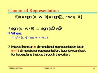
Canonical Representation f(x) = sgn {x  ¢  w -   } = sgn{  i=1 n  w i  x i  -   } sgn {x  ¢  w -   }  ´   sgn {x’  ¢  w’}  Where:  x’ = (x, -  )  and w’ = (w,1)  Moved from an  n  dimensional representation to an  (n+1)  dimensional representation, but now can look for hyperplans that go through the origin.
LMS: An online, local search algorithm A local search learning algorithm requires: Hypothesis Space:  Linear Threshold Units Loss function:  Squared loss  LMS  (Least Mean Square, L 2 ) Search procedure:  Gradient Descent w 
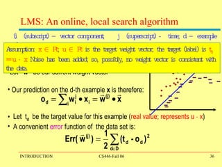
LMS: An online, local search algorithm Let  w (j)  be our current weight vector Our prediction on the d-th example  x  is therefore: Let  t d   be the target value for this example ( real value; represents u  ¢  x ) A convenient  error  function of  the data set is: (i  (subscript) – vector component;  j  (superscript) -  time; d – example #) Assumption:  x  2  R n ;  u  2  R n  is the target weight vector; the target (label) is  t d  = u  ¢  x  Noise has been added; so, possibly, no weight vector is consistent with the data.
Gradient Descent We use gradient descent to determine the weight vector that minimizes  Err (w)  ; Fixing the set D of examples, E is a function of  w j At each step, the weight vector is modified in the direction that produces the steepest descent along the error surface . E(w) w w 4  w 3  w 2  w 1
To find the best direction in the  weight  space  we compute the gradient  of  E  with respect to each of the components of  This vector specifies the direction that produces the steepest  increase in E; We want to modify  in the direction of Where:  Gradient Descent
We have:  Therefore:  Gradient Descent: LMS
Gradient Descent: LMS Weight update rule:
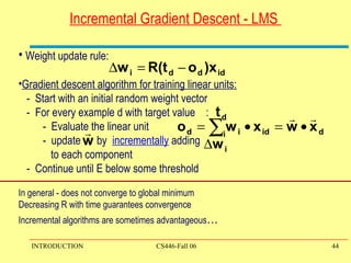
Gradient Descent: LMS Weight update rule: Gradient descent algorithm for training linear units: -  Start with an initial random weight vector -  For every example d with target value  : -  Evaluate the linear unit -  update  by adding  to each component -  Continue until E below some threshold
Weight update rule: Gradient descent algorithm for training linear units: -  Start with an initial random weight vector -  For every example d with target value  : -  Evaluate the linear unit -  update  by adding  to each component -  Continue until E below some threshold  Because the surface contains only a single global minimum the algorithm will converge to a weight vector with minimum error, regardless of whether the examples are linearly separable Gradient Descent: LMS
Weight update rule: Incremental Gradient Descent: LMS
Incremental Gradient Descent - LMS  Weight update rule: Gradient descent algorithm for training linear units: -  Start with an initial random weight vector -  For every example d with target value  : -  Evaluate the linear unit -  update  by  incrementally  adding  to each component  -  Continue until E below some threshold  In general - does not converge to global minimum Decreasing R with time guarantees convergence  Incremental algorithms are sometimes advantageous …
Learning Rates and Convergence In the general (non-separable) case the learning rate R  must decrease to  zero to guarantee convergence. It cannot    decrease too quickly nor too slowly.  The learning rate is called the  step size.  There are more  sophisticates  algorithms (Conjugate Gradient)  that choose  the step size automatically and converge faster. There is only one “basin” for linear threshold units, so a  local minimum is the global minimum. However, choosing  a starting point can make the algorithm converge much  faster.
Computational Issues Assume the data is linearly separable. Sample complexity: Suppose we want to ensure that our LTU has an error rate  (on new examples) of less than    with high probability(at least (1-  )) How large must m (the number of examples) be in order to  achieve this? It can be shown that for  n  dimensional problems m = O(1/    [ln(1/   ) + (n+1) ln(1/   ) ]. Computational complexity: What can be said? It can be shown that there exists a polynomial time algorithm for  finding  consistent LTU (by reduction from linear programming).  (On-line algorithms have inverse quadratic dependence on the margin)
Other methods for LTUs Direct Computation:  Set   J( w ) = 0 and solve for  w  . Can be accomplished using SVD  methods. Fisher Linear Discriminant: A direct computation method.  Probabilistic  methods (naive Bayes): Produces a stochastic classifier that can be viewed as a linear  threshold unit. Winnow:  A multiplicative update algorithm with the property that it can  handle  large  numbers of irrelevant attributes.
Summary of LMS algorithms for LTUs Local search:  Begins with initial weight vector. Modifies iteratively to minimize and error function. The error function is  loosely  related to the goal of  minimizing the number of classification errors.  Memory:  The classifier is constructed from the training examples.  The examples can then be discarded. Online or Batch: Both online and batch variants of the algorithms can be used.
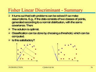
Fisher Linear Discriminant This is a classical method for discriminant analysis. It is based on dimensionality reduction – finding a better representation for the data. Notice that just finding good representations for the data may  not always be good for discrimination . [E.g., O, Q] Intuition:  Consider projecting data from  d  dimensions to the line.   Likely results in a mixed set of points and  poor separation. However, by  moving the line around  we might be able to find an orientation for which the projected samples are well separated.
Fisher Linear Discriminant Sample S= {x 1 , x 2 , … x n  }  2   < d P, N are the positive, negative examples, resp. Let  w   2   < d . And assume  ||w||=1.  Then:  The projection of a vector  x  on a line in the direction w,  is  w t   ¢  x . If the data is linearly separable, there exists a good direction  w . (all vectors are column vectors)
Finding a Good Direction Sample mean (positive, P; Negative, N):  M p  = 1/|P|   P  x i The mean of the projected (positive, negative) points m p  = 1/|P|   P  w t   ¢  x i = 1/|P|   P  y i  = w t   ¢  M p Is simply the projection of the sample mean.  Therefore, the distance between the projected means is: |m p  -   m N |= |w t   ¢  (M p -  M N  )| Want large difference
Finding a Good Direction (2) Scaling  w  isn’t the solution. We want the difference to be large relative to some measure of standard deviation for each class.  S 2 p  =   P  (y-m p  ) 2  s 2 N  =   N  (y-m N  ) 2 1/ (  S 2 p  +   s 2 N  )  within class scatter : estimates the variances of the sample.  The  Fischer linear discriminant  employs the linear function w t   ¢  x for which J(w) = | m P  – m N | 2  / S 2 p  + s 2 N   is maximized. How to make this a classifier?  How to find the optimal w?  Some Algebra
J as an explicit function of w (1) Compute the scatter matrices:  S p  =   P  (x-M p  )(x-M p  ) t  S N  =   N  (x-M N  )(x-M N  ) t  and  S W  = S p  + S p   We can write:  S 2 p  =   P  (y-m p  ) 2  =   P  (w t  x -w t  M p  ) 2  =  =   P  w t  (x- M p  )   (x- M p  ) t  w = w t  S p   w  Therefore: S 2 p  + S 2 N  = w t  S W   w   S W  is the within-class scatter matrix. It is proportional to the sample covariance matrix for the d-dimensional sample.
J as an explicit function of w (2) We can do a similar computation for the means: S B  = (M P -M N  )(M P -M N  ) t and we can write:  (m P -m N  ) 2  =  (w t  M P -w t  M N  ) 2  =  =  w t  (M P -M N )   (M P -M N )  t  w = w t  S B   w  Therefore: S B  is the  between-class scatter matrix . It is the outer product of two vectors and therefore its rank is at most 1.  S B   w  is always in the direction of (M P -M N  )
J as an explicit function of w (3) Now we can compute explicitly: We can do a similar computation for the means: J(w) =  | m P  – m N | 2  / S 2 p  + s 2 N   = w t  S B   w / w t  S W   w   We are looking for a the value of  w  that maximizes this expression. This is a generalized eigenvalue problem; when  S W  is nonsingular, it is just a eigenvalue problem. The solution can be written without solving the problem, as:  w=S -1 W   (M P -M N  ) This is the Fisher Linear Discriminant . 1 : We converted a d-dimensional problem to a 1-dimensional problem and suggested a solution that  makes some sense. 2:  We have a solution that makes sense; how to make it a classifier? And, how good it is?
Fisher Linear Discriminant - Summary It turns out that both problems can be solved if we make assumptions. E.g., if the data consists of two classes of points, generated according to a normal distribution, with the same covariance. Then: The solution is optimal. Classification can be done by choosing a threshold, which can be computed. Is this satisfactory?
Introduction - Summary We introduced the technical part of the class by giving two examples for (very different) approaches to linear discrimination. There are many other solutions. Questions 1 : But this assumes that we are linear. Can we learn a function that is more flexible in terms of what it does with the features space? Question 2 : Can we say something about the quality of what we learn (sample complexity, time complexity; quality)

ppt

  • 1.
    CS 446: Machine Learning Gerald DeJong [email_address] 3-0491 3320 SC Recent approval for a TA to be named later
  • 2.
    Office hours: aftermost classes and Thur @ 3 Text: Mitchell’s Machine Learning Midterm: Oct. 4 Final: Dec. 12 each a third Homeworks / projects Submit at the beginning of class Late penalty: 20% / day up to 3 days Programming, some in-class assignments Class web site soon Cheating: none allowed! We adopt dept. policy
  • 3.
    Please answer theseand hand in now Name Department Where (If?*) you had Intro AI course Who taught it (esp. if not here) 1) Why interested in Machine Learning? 2) Any topics you would like to see covered? * may require significant additional effort
  • 4.
    Approx. Course Overview/ Topics Introduction: Basic problems and questions A detailed examples: Linear threshold units Basic Paradigms: PAC (Risk Minimization); Bayesian Theory; SRM (Structural Risk Minimization); Compression; Maximum Entropy;… Generative/Discriminative; Classification/Skill;… Learning Protocols Online/Batch; Supervised/Unsupervised/Semi-supervised; Delayed supervision Algorithms: Decision Trees (C4.5) [Rules and ILP (Ripper, Foil)] Linear Threshold Units (Winnow, Perceptron; Boosting; SVMs; Kernels) Probabilistic Representations (naïve Bayes, Bayesian trees; density estimation) Delayed supervision: RL Unsupervised/Semi-supervised: EM Clustering, Dimensionality Reduction, or others of student interest
  • 5.
    What to LearnClassifiers: Learn a hidden function Concept Learning: chair ? face ? game ? Diagnosis: medical; risk assessment Models: Learn a map (and use it to navigate) Learn a distribution (and use it to answer queries) Learn a language model; Learn an Automaton Skills: Learn to play games; Learn a Plan / Policy Learn to Reason; Learn to Plan Clusterings: Shapes of objects; Functionality; Segmentation Abstraction Focus on classification (importance, theoretical richness, generality,…)
  • 6.
    What to Learn? Direct Learning: (discriminative, model-free[bad name]) Learn a function that maps an input instance to the sought after property. Model Learning: (indirect, generative) Learning a model of the domain; then use it to answer various questions about the domain In both cases, several protocols can be used – Supervised – learner is given examples and answers Unsupervised – examples, but no answers Semi-supervised – some examples w/answers, others w/o Delayed supervision
  • 7.
    Supervised LearningGiven: Examples (x,f ( x)) of some unknown function f Find: A good approximation to f x provides some representation of the input The process of mapping a domain element into a representation is called Feature Extraction. (Hard; ill-understood; important) x 2 {0,1} n or x 2 < n The target function (label) f(x) 2 {-1,+1} Binary Classification f(x) 2 {1,2,3,.,k-1} Multi-class classification f(x) 2 < Regression
  • 8.
    Example and HypothesisSpaces X H X: Example Space – set of all well-formed inputs [w/a distribution] H: Hypothesis Space – set of all well-formed outputs - - + + + - - - +
  • 9.
    Supervised Learning:Examples Disease diagnosis x: Properties of patient (symptoms, lab tests) f : Disease (or maybe: recommended therapy) Part-of-Speech tagging x: An English sentence (e.g., The can will rust) f : The part of speech of a word in the sentence Face recognition x: Bitmap picture of person’s face f : Name the person (or maybe: a property of) Automatic Steering x: Bitmap picture of road surface in front of car f : Degrees to turn the steering wheel
  • 10.
    y = f (x 1 , x 2 , x 3 , x 4 ) Unknown function x 1 x 2 x 3 x 4 A Learning Problem X H ? ? (Boolean: x1, x2, x3, x4, f )
  • 11.
    y = f (x 1 , x 2 , x 3 , x 4 ) Unknown function x 1 x 2 x 3 x 4 Training Set Example x 1 x 2 x 3 x 4 y 1 0 0 1 0 0 3 0 0 1 1 1 4 1 0 0 1 1 5 0 1 1 0 0 6 1 1 0 0 0 7 0 1 0 1 0 2 0 1 0 0 0
  • 12.
    Hypothesis Space CompleteIgnorance: How many possible functions? 2 16 = 56536 over four input features. After seven examples how many possibilities for f? 2 9 possibilities remain for f How many examples until we figure out which is correct? We need to see labels for all 16 examples! Is Learning Possible? Example x 1 x 2 x 3 x 4 y 1 1 1 1 ? 0 0 0 0 ? 1 0 0 0 ? 1 0 1 1 ? 1 1 0 0 0 1 1 0 1 ? 1 0 1 0 ? 1 0 0 1 1 0 1 0 0 0 0 1 0 1 0 0 1 1 0 0 0 1 1 1 ? 0 0 1 1 1 0 0 1 0 0 0 0 0 1 ? 1 1 1 0 ?
  • 13.
    Another Hypothesis SpaceSimple Rules: There are only 16 simple conjunctive rules of the form y=x i Æ x j Æ x k ... No simple rule explains the data. The same is true for simple clauses 1 0 0 1 0 0 3 0 0 1 1 1 4 1 0 0 1 1 5 0 1 1 0 0 6 1 1 0 0 0 7 0 1 0 1 0 2 0 1 0 0 0 y =c x 1 1100 0 x 2 0100 0 x 3 0110 0 x 4 0101 1 x 1  x 2 1100 0 x 1  x 3 0011 1 x 1  x 4 0011 1 Rule Counterexample x 2  x 3 0011 1 x 2  x 4 0011 1 x 3  x 4 1001 1 x 1  x 2  x 3 0011 1 x 1  x 2  x 4 0011 1 x 1  x 3  x 4 0011 1 x 2  x 3  x 4 0011 1 x 1  x 2  x 3  x 4 0011 1 Rule Counterexample
  • 14.
    Third Hypothesis Spacem-of-n rules: There are 29 possible rules of the form ”y = 1 if and only if at least m of the following n variables are 1” Found a consistent hypothesis. 1 0 0 1 0 0 3 0 0 1 1 1 4 1 0 0 1 1 5 0 1 1 0 0 6 1 1 0 0 0 7 0 1 0 1 0 2 0 1 0 0 0  x 1  3 - - -  x 2  2 - - -  x 3  1 - - -  x 4  7 - - -  x 1, x 2  2 3 - -  x 1, x 3  1 3 - -  x 1, x 4  6 3 - -  x 2, x 3  2 3 - - variables 1 -of 2 -of 3 -of 4 -of  x 2, x 4  2 3 - -  x 3, x 4  4 4 - -  x 1, x 2, x 3  1 3 3 -  x 1, x 2, x 4  2 3 3 -  x 1, x 3, x 4  1    3 -  x 2, x 3, x 4  1 5 3 -  x 1, x 2, x 3, x 4  1 5 3 3 variables 1 -of 2 -of 3 -of 4 -of
  • 15.
    Views of LearningLearning is the removal of our remaining uncertainty: Suppose we knew that the unknown function was an m-of-n Boolean function, then we could use the training data to infer which function it is. Learning requires guessing a good, small hypothesis class : We can start with a very small class and enlarge it until it contains an hypothesis that fits the data. We could be wrong ! Our prior knowledge might be wrong: y=x4  one-of (x1, x3) is also consistent Our guess of the hypothesis class could be wrong If this is the unknown function, then we will make errors when we are given new examples, and are asked to predict the value of the function
  • 16.
    General strategy forMachine Learning H should respect our prior understanding: Excess expressivity makes learning difficult Expressivity of H should match our ignorance Understand flexibility of std. hypothesis spaces: Decision trees, neural networks, rule grammars, stochastic models Hypothesis spaces of flexible size; Nested collections of hypotheses. ML succeeds when these interrelate Develop algorithms for finding a hypothesis h that fits the data h will likely perform well when the richness of H is less than the information in the training set
  • 17.
    Terminology Training example: An pair of the form (x, f (x)) Target function (concept): The true function f (?) Hypothesis: A proposed function h, believed to be similar to f. Concept: Boolean function. Example for which f (x)= 1 are positive examples; those for which f (x)= 0 are negative examples (instances) (sometimes used interchangeably w/ “Hypothesis”) Classifier: A discrete valued function. The possible value of f: {1,2,…K} are the classes or class labels . Hypothesis space: The space of all hypotheses that can, in principle, be output by the learning algorithm. Version Space: The space of all hypothesis in the hypothesis space that have not yet been ruled out.
  • 18.
    Key Issues inMachine Learning Modeling How to formulate application problems as machine learning problems ? Learning Protocols (where is the data coming from, how?) Project examples: [complete products] EMAIL Given a seminar announcement, place the relevant information in my outlook Given a message, place it in the appropriate folder Image processing: Given a folder with pictures; automatically rotate all those that need it. My office: have my office greet me in the morning and unlock the door (but do it only for me!) Context Sensitive Spelling: Incorporate into Word
  • 19.
    Key Issues inMachine Learning Modeling How to formulate application problems as machine learning problems ? Learning Protocols (where is the data coming from, how?) Representation: What are good hypothesis spaces ? Any rigorous way to find these? Any general approach? Algorithms: What are good algorithms? How do we define success? Generalization Vs. over fitting The computational problem
  • 20.
    Example: Generalization vsOverfitting What is a Tree ? A botanist Her brother A tree is something with A tree is a green thing leaves I’ve seen before Neither will generalize well
  • 21.
    Self-organize into Groupsof 4 or 5 Assignment 1 The Badges Game …… Prediction or Modeling? Representation Background Knowledge When did learning take place? Learning Protocol? What is the problem? Algorithms
  • 22.
    Linear Discriminators Idon’t know { whether, weather} to laugh or cry How can we make this a learning problem? We will look for a function F: Sentences  { whether, weather} We need to define the domain of this function better. An option : For each word w in English define a Boolean feature x w : [x w =1] iff w is in the sentence This maps a sentence to a point in {0,1} 50,000 In this space: some points are whether points some are weather points Learning Protocol? Supervised? Unsupervised?
  • 23.
    What’s Good? Learning problem : Find a function that best separates the data What function? What’s best? How to find it? A possibility: Define the learning problem to be: Find a (linear) function that best separates the data
  • 24.
    Exclusive-OR (XOR)(x 1 Æ x 2) Ç ( : {x 1 } Æ : {x 2 }) In general: a parity function. x i 2 {0,1} f(x 1 , x 2 ,…, x n ) = 1 iff  x i is even This function is not linearly separable . x 1 x 2
  • 25.
    Sometimes Functions Canbe Made Linear x 1 x 2 x 4 Ç x 2 x 4 x 5 Ç x 1 x 3 x 7 Space: X= x 1 , x 2 ,…, x n input Transformation New Space: Y = {y 1 ,y 2 ,…} = {x i ,x i x j , x i x j x j } y 3 Ç y 4 Ç y 7 New discriminator is functionally simpler Weather Whether
  • 26.
    Data are notseparable in one dimension Not separable if you insist on using a specific class of functions Feature Space x
  • 27.
    Blown Up FeatureSpace Data are separable in <x, x 2 > space x x 2 Key issue: what features to use. Computationally, can be done implicitly (kernels)
  • 28.
    A General Frameworkfor Learning Goal: predict an unobserved output value y 2 Y based on an observed input vector x 2 X Estimate a functional relationship y~f(x) from a set {(x,y) i } i=1,n Most relevant - Classification : y  {0,1} (or y  {1,2,…k} ) (But, within the same framework can also talk about Regression, y 2 < What do we want f(x) to satisfy? We want to minimize the Loss (Risk): L(f()) = E X,Y ( [f(x)  y] ) Where: E X,Y denotes the expectation with respect to the true distribution . Simply: # of mistakes […] is a indicator function
  • 29.
    A General Frameworkfor Learning (II) We want to minimize the Loss: L(f()) = E X,Y ( [f(X)  Y] ) Where: E X,Y denotes the expectation with respect to the true distribution . We cannot do that. Why not? Instead, we try to minimize the empirical classification error. For a set of training examples {(X i ,Y i )} i=1,n Try to minimize the observed loss (Issue I : when is this good enough? Not now) This minimization problem is typically NP hard. To alleviate this computational problem, minimize a new function – a convex upper bound of the classification error function I (f(x),y) =[f(x)  y] = {1 when f(x)  y; 0 otherwise}
  • 30.
    Learning as anOptimization Problem A Loss Function L(f(x),y) measures the penalty incurred by a classifier f on example (x,y). There are many different loss functions one could define: Misclassification Error: L(f(x),y) = 0 if f(x) = y; 1 otherwise Squared Loss: L(f(x),y) = (f(x) –y) 2 Input dependent loss: L(f(x),y) = 0 if f(x)= y; c(x)otherwise. A continuous convex loss function also allows a conceptually simple optimization algorithm. f(x) –y
  • 31.
    How to Learn? Local search: Start with a linear threshold function. See how well you are doing. Correct Repeat until you converge. There are other ways that do not search directly in the hypotheses space Directly compute the hypothesis?
  • 32.
    Learning Linear Separators(LTU) f(x) = sgn {x ¢ w -  } = sgn{  i=1 n w i x i -  } x= ( x 1 ,x 2 ,… ,x n ) 2 {0,1} n is the feature based encoding of the data point w= ( w 1 ,w 2 ,… ,w n ) 2 < n is the target function.  determines the shift with respect to the origin w 
  • 33.
    Expressivity f(x)= sgn {x ¢ w -  } = sgn{  i=1 n w i x i -  } Many functions are Linear Conjunctions: y = x 1 Æ x 3 Æ x 5 y = sgn{1 ¢ x 1 + 1 ¢ x 3 + 1 ¢ x 5 - 3} At least m of n: y = at least 2 of { x 1 ,x 3 , x 5 } y = sgn{1 ¢ x 1 + 1 ¢ x 3 + 1 ¢ x 5 - 2} Many functions are not Xor: y = x 1 Æ x 2 Ç x 1 Æ x 2 Non trivial DNF: y = x 1 Æ x 2 Ç x 3 Æ x 4 But some can be made linear Probabilistic Classifiers as well
  • 34.
    Canonical Representation f(x)= sgn {x ¢ w -  } = sgn{  i=1 n w i x i -  } sgn {x ¢ w -  } ´ sgn {x’ ¢ w’} Where: x’ = (x, -  ) and w’ = (w,1) Moved from an n dimensional representation to an (n+1) dimensional representation, but now can look for hyperplans that go through the origin.
  • 35.
    LMS: An online,local search algorithm A local search learning algorithm requires: Hypothesis Space: Linear Threshold Units Loss function: Squared loss LMS (Least Mean Square, L 2 ) Search procedure: Gradient Descent w 
  • 36.
    LMS: An online,local search algorithm Let w (j) be our current weight vector Our prediction on the d-th example x is therefore: Let t d be the target value for this example ( real value; represents u ¢ x ) A convenient error function of the data set is: (i (subscript) – vector component; j (superscript) - time; d – example #) Assumption: x 2 R n ; u 2 R n is the target weight vector; the target (label) is t d = u ¢ x Noise has been added; so, possibly, no weight vector is consistent with the data.
  • 37.
    Gradient Descent Weuse gradient descent to determine the weight vector that minimizes Err (w) ; Fixing the set D of examples, E is a function of w j At each step, the weight vector is modified in the direction that produces the steepest descent along the error surface . E(w) w w 4 w 3 w 2 w 1
  • 38.
    To find thebest direction in the weight space we compute the gradient of E with respect to each of the components of This vector specifies the direction that produces the steepest increase in E; We want to modify in the direction of Where: Gradient Descent
  • 39.
    We have: Therefore: Gradient Descent: LMS
  • 40.
    Gradient Descent: LMSWeight update rule:
  • 41.
    Gradient Descent: LMSWeight update rule: Gradient descent algorithm for training linear units: - Start with an initial random weight vector - For every example d with target value : - Evaluate the linear unit - update by adding to each component - Continue until E below some threshold
  • 42.
    Weight update rule:Gradient descent algorithm for training linear units: - Start with an initial random weight vector - For every example d with target value : - Evaluate the linear unit - update by adding to each component - Continue until E below some threshold Because the surface contains only a single global minimum the algorithm will converge to a weight vector with minimum error, regardless of whether the examples are linearly separable Gradient Descent: LMS
  • 43.
    Weight update rule:Incremental Gradient Descent: LMS
  • 44.
    Incremental Gradient Descent- LMS Weight update rule: Gradient descent algorithm for training linear units: - Start with an initial random weight vector - For every example d with target value : - Evaluate the linear unit - update by incrementally adding to each component - Continue until E below some threshold In general - does not converge to global minimum Decreasing R with time guarantees convergence Incremental algorithms are sometimes advantageous …
  • 45.
    Learning Rates andConvergence In the general (non-separable) case the learning rate R must decrease to zero to guarantee convergence. It cannot decrease too quickly nor too slowly. The learning rate is called the step size. There are more sophisticates algorithms (Conjugate Gradient) that choose the step size automatically and converge faster. There is only one “basin” for linear threshold units, so a local minimum is the global minimum. However, choosing a starting point can make the algorithm converge much faster.
  • 46.
    Computational Issues Assumethe data is linearly separable. Sample complexity: Suppose we want to ensure that our LTU has an error rate (on new examples) of less than  with high probability(at least (1-  )) How large must m (the number of examples) be in order to achieve this? It can be shown that for n dimensional problems m = O(1/  [ln(1/  ) + (n+1) ln(1/  ) ]. Computational complexity: What can be said? It can be shown that there exists a polynomial time algorithm for finding consistent LTU (by reduction from linear programming). (On-line algorithms have inverse quadratic dependence on the margin)
  • 47.
    Other methods forLTUs Direct Computation: Set  J( w ) = 0 and solve for w . Can be accomplished using SVD methods. Fisher Linear Discriminant: A direct computation method. Probabilistic methods (naive Bayes): Produces a stochastic classifier that can be viewed as a linear threshold unit. Winnow: A multiplicative update algorithm with the property that it can handle large numbers of irrelevant attributes.
  • 48.
    Summary of LMSalgorithms for LTUs Local search: Begins with initial weight vector. Modifies iteratively to minimize and error function. The error function is loosely related to the goal of minimizing the number of classification errors. Memory: The classifier is constructed from the training examples. The examples can then be discarded. Online or Batch: Both online and batch variants of the algorithms can be used.
  • 49.
    Fisher Linear DiscriminantThis is a classical method for discriminant analysis. It is based on dimensionality reduction – finding a better representation for the data. Notice that just finding good representations for the data may not always be good for discrimination . [E.g., O, Q] Intuition: Consider projecting data from d dimensions to the line. Likely results in a mixed set of points and poor separation. However, by moving the line around we might be able to find an orientation for which the projected samples are well separated.
  • 50.
    Fisher Linear DiscriminantSample S= {x 1 , x 2 , … x n } 2 < d P, N are the positive, negative examples, resp. Let w 2 < d . And assume ||w||=1. Then: The projection of a vector x on a line in the direction w, is w t ¢ x . If the data is linearly separable, there exists a good direction w . (all vectors are column vectors)
  • 51.
    Finding a GoodDirection Sample mean (positive, P; Negative, N): M p = 1/|P|  P x i The mean of the projected (positive, negative) points m p = 1/|P|  P w t ¢ x i = 1/|P|  P y i = w t ¢ M p Is simply the projection of the sample mean. Therefore, the distance between the projected means is: |m p - m N |= |w t ¢ (M p - M N )| Want large difference
  • 52.
    Finding a GoodDirection (2) Scaling w isn’t the solution. We want the difference to be large relative to some measure of standard deviation for each class. S 2 p =  P (y-m p ) 2 s 2 N =  N (y-m N ) 2 1/ ( S 2 p + s 2 N ) within class scatter : estimates the variances of the sample. The Fischer linear discriminant employs the linear function w t ¢ x for which J(w) = | m P – m N | 2 / S 2 p + s 2 N is maximized. How to make this a classifier? How to find the optimal w? Some Algebra
  • 53.
    J as anexplicit function of w (1) Compute the scatter matrices: S p =  P (x-M p )(x-M p ) t S N =  N (x-M N )(x-M N ) t and S W = S p + S p We can write: S 2 p =  P (y-m p ) 2 =  P (w t x -w t M p ) 2 = =  P w t (x- M p ) (x- M p ) t w = w t S p w Therefore: S 2 p + S 2 N = w t S W w S W is the within-class scatter matrix. It is proportional to the sample covariance matrix for the d-dimensional sample.
  • 54.
    J as anexplicit function of w (2) We can do a similar computation for the means: S B = (M P -M N )(M P -M N ) t and we can write: (m P -m N ) 2 = (w t M P -w t M N ) 2 = = w t (M P -M N ) (M P -M N ) t w = w t S B w Therefore: S B is the between-class scatter matrix . It is the outer product of two vectors and therefore its rank is at most 1. S B w is always in the direction of (M P -M N )
  • 55.
    J as anexplicit function of w (3) Now we can compute explicitly: We can do a similar computation for the means: J(w) = | m P – m N | 2 / S 2 p + s 2 N = w t S B w / w t S W w We are looking for a the value of w that maximizes this expression. This is a generalized eigenvalue problem; when S W is nonsingular, it is just a eigenvalue problem. The solution can be written without solving the problem, as: w=S -1 W (M P -M N ) This is the Fisher Linear Discriminant . 1 : We converted a d-dimensional problem to a 1-dimensional problem and suggested a solution that makes some sense. 2: We have a solution that makes sense; how to make it a classifier? And, how good it is?
  • 56.
    Fisher Linear Discriminant- Summary It turns out that both problems can be solved if we make assumptions. E.g., if the data consists of two classes of points, generated according to a normal distribution, with the same covariance. Then: The solution is optimal. Classification can be done by choosing a threshold, which can be computed. Is this satisfactory?
  • 57.
    Introduction - SummaryWe introduced the technical part of the class by giving two examples for (very different) approaches to linear discrimination. There are many other solutions. Questions 1 : But this assumes that we are linear. Can we learn a function that is more flexible in terms of what it does with the features space? Question 2 : Can we say something about the quality of what we learn (sample complexity, time complexity; quality)

Editor's Notes

  • #5 As we said, this is the game we are playing; in NLP, it has always been clear, that the raw information In a sentence is not sufficient, as is to represent a good predictor. Better functions of the input were Generated, and learning was done in these terms.
  • #6 As we said, this is the game we are playing; in NLP, it has always been clear, that the raw information In a sentence is not sufficient, as is to represent a good predictor. Better functions of the input were Generated, and learning was done in these terms.
  • #7 As we said, this is the game we are playing; in NLP, it has always been clear, that the raw information In a sentence is not sufficient, as is to represent a good predictor. Better functions of the input were Generated, and learning was done in these terms.
  • #8 Badges game Don’t give me the answer Start thinking about how to write a program that will figure out whether my name has + or – next to it.
  • #10 Badges game Don’t give me the answer Start thinking about how to write a program that will figure out whether my name has + or – next to it.
  • #13 Badges game Don’t give me the answer Start thinking about how to write a program that will figure out whether my name has + or – next to it.
  • #14 Badges game Don’t give me the answer Start thinking about how to write a program that will figure out whether my name has + or – next to it.
  • #15 Badges game Don’t give me the answer Start thinking about how to write a program that will figure out whether my name has + or – next to it.
  • #16 Badges game Don’t give me the answer Start thinking about how to write a program that will figure out whether my name has + or – next to it.
  • #17 Badges game Don’t give me the answer Start thinking about how to write a program that will figure out whether my name has + or – next to it.
  • #18 Badges game Don’t give me the answer Start thinking about how to write a program that will figure out whether my name has + or – next to it.
  • #19 Badges game Don’t give me the answer Start thinking about how to write a program that will figure out whether my name has + or – next to it.
  • #20 Badges game Don’t give me the answer Start thinking about how to write a program that will figure out whether my name has + or – next to it.
  • #21 Badges game Don’t give me the answer Start thinking about how to write a program that will figure out whether my name has + or – next to it.
  • #22 Badges game Don’t give me the answer Start thinking about how to write a program that will figure out whether my name has + or – next to it.
  • #23 As we said, this is the game we are playing; in NLP, it has always been clear, that the raw information In a sentence is not sufficient, as is to represent a good predictor. Better functions of the input were Generated, and learning was done in these terms.
  • #24 As we said, this is the game we are playing; in NLP, it has always been clear, that the raw information In a sentence is not sufficient, as is to represent a good predictor. Better functions of the input were Generated, and learning was done in these terms.
  • #25 As we said, this is the game we are playing; in NLP, it has always been clear, that the raw information In a sentence is not sufficient, as is to represent a good predictor. Better functions of the input were Generated, and learning was done in these terms.
  • #26 As we said, this is the game we are playing; in NLP, it has always been clear, that the raw information In a sentence is not sufficient, as is to represent a good predictor. Better functions of the input were Generated, and learning was done in these terms.
  • #29 As we said, this is the game we are playing; in NLP, it has always been clear, that the raw information In a sentence is not sufficient, as is to represent a good predictor. Better functions of the input were Generated, and learning was done in these terms.
  • #30 As we said, this is the game we are playing; in NLP, it has always been clear, that the raw information In a sentence is not sufficient, as is to represent a good predictor. Better functions of the input were Generated, and learning was done in these terms.
  • #31 As we said, this is the game we are playing; in NLP, it has always been clear, that the raw information In a sentence is not sufficient, as is to represent a good predictor. Better functions of the input were Generated, and learning was done in these terms.
  • #37 Good treatment in Bishop, Chp 3 Classic Weiner filtering solution; text omits 0.5 factor; In any case we use the gradient and eta (text) or R (these notes) to modulate the step size
  • #50 Badges game Don’t give me the answer Start thinking about how to write a program that will figure out whether my name has + or – next to it.
  • #51 Badges game Don’t give me the answer Start thinking about how to write a program that will figure out whether my name has + or – next to it.
  • #52 Badges game Don’t give me the answer Start thinking about how to write a program that will figure out whether my name has + or – next to it.
  • #53 Badges game Don’t give me the answer Start thinking about how to write a program that will figure out whether my name has + or – next to it.
  • #54 Badges game Don’t give me the answer Start thinking about how to write a program that will figure out whether my name has + or – next to it.
  • #55 Badges game Don’t give me the answer Start thinking about how to write a program that will figure out whether my name has + or – next to it.
  • #56 Badges game Don’t give me the answer Start thinking about how to write a program that will figure out whether my name has + or – next to it.
  • #57 Badges game Don’t give me the answer Start thinking about how to write a program that will figure out whether my name has + or – next to it.
  • #58 Badges game Don’t give me the answer Start thinking about how to write a program that will figure out whether my name has + or – next to it.