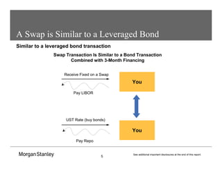
- Interest rate swaps allow parties to exchange interest rate cash flows, with one party paying fixed rates and the other floating rates tied to a reference rate like LIBOR.
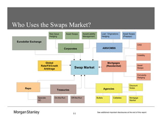
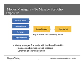
- Corporations, money managers, mortgage holders, and dealers use swaps to hedge interest rate risks and manage portfolio exposures.
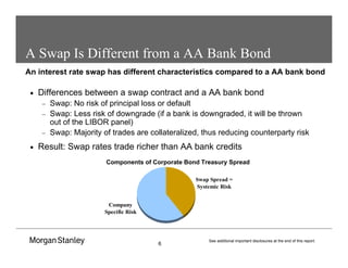
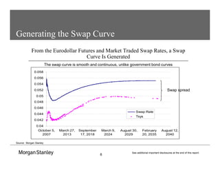
- The swap spread, the difference between Treasury yields and swap fixed rates, is influenced by factors like funding costs and supply/demand dynamics.
- Forward-starting swaps allow market participants to express views on future interest rate movements over a specific time horizon.
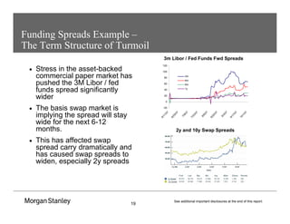
The Cross Section of Realized Stock Returns: The Pre-COMPUSTAT EvidenceSudarshan Kadariya
Â
This study analyzed the explanatory power of various financial variables on the cross-sectional variation in stock returns between 1940-1960 using data from Moody's Industrial Manuals and CRSP. The study found:
1) Book-to-market equity, earnings yield, and cash flow yield had significant explanatory power for predicting subsequent stock returns, especially in January.
2) There was a strong seasonal effect, with these variables exhibiting stronger predictive ability for returns in January than the rest of the year.
3) Other variables like historical beta, firm size, and sales growth had weaker or insignificant ability to explain cross-sectional differences in returns.
Delta measures the change in a portfolio based on the change in the price of the underlying asset. Gamma measures the rate of change of delta based on price changes. Vega measures the change in value based on changes in volatility. Theta measures the daily time-based decay in value. Rho measures the change in value due to interest rate changes. Delta hedging involves buying and selling the underlying asset to maintain a delta-neutral position as the delta changes over time. Gamma and vega hedging require taking positions in options or other derivatives. Traders aim to keep their portfolios delta-neutral daily and control gamma and vega within risk limits.
Derivatives are financial contracts whose value is derived from an underlying asset. The three main types are forwards, futures, and options. Forwards and futures obligate the buyer to purchase an asset at a future date at a preset price. Options provide the right, but not obligation, for the buyer to purchase or sell the asset. Derivatives allow participants to hedge or speculate on price movements in the underlying asset. Major global futures exchanges include CME, CBOT, NYMEX, and EUREX.
This document discusses interest rate swaps. It defines an interest rate swap as an agreement to exchange interest rate payments, with one leg fixed and the other floating. Common types include paying fixed rate interest to receive floating, and vice versa. Interest rate swaps are used to hedge against rising or falling interest rates by transforming fixed deposits/borrowings to floating, or floating to fixed. Examples show how swaps can benefit entities by reducing income/funding costs if rates move in the desired direction.
The document discusses the Value-at-Risk (VaR) measure which estimates the maximum potential loss of a portfolio over a given time period at a certain confidence level. It outlines some key parameters used in calculating VaR such as the sampling period, analysis horizon, and sampling frequency. The document also differentiates between relative VaR, marginal VaR, and conditional VaR which are related but distinct VaR measures. Finally, it provides an overview of different VaR methodologies including historical simulation, parametric simulation, and Monte Carlo simulation which will be explored in more detail later.
This document provides an overview of convertible bonds, including:
1) Key terms like conversion ratio and conversion price as well as how the price of a convertible bond is calculated.
2) The hybrid characteristics of convertibles that provide downside protection like bonds and upside potential like equities.
3) Metrics used to analyze convertibles such as delta, gamma, and cheapness.
4) An example of a hypothetical Concerto-FS convertible bond is presented to demonstrate these concepts.
We cannot reduce market risks or systematic risks but we can have a measure of these risks with the help of beta.
With the help of beta we can approximately tell how much a particular stock will move if we know how much the whole stock market is going to move.
ďşPlease Subscribe to this Channel for more solutions and lectures
http://www.youtube.com/onlineteaching
Chapter 5: Discrete Probability Distribution
5.1: Probability Distribution
The document discusses the Capital Asset Pricing Model (CAPM). It defines systematic and unsystematic risk, the beta coefficient as a measure of systematic risk, and outlines the key assumptions and formula of CAPM. The Security Market Line (SML) graphs the relationship between risk and return predicted by CAPM. Some limitations of CAPM are that it assumes variance captures all risk and homogeneous investor expectations. Alternatives to CAPM discussed include Consumption CAPM, Intertemporal CAPM, and Arbitrage Pricing Theory.
This document provides an overview of a seminar on financial markets from Saunders Learning Group. The seminar aims to provide a simple guide to investing in financial securities and how financial markets work. Saunders Learning Group offers various training programs, workshops and seminars targeted towards the financial services industry.
L2 flash cards portfolio management - SS 18analystbuddy
Â
Mean-variance analysis is used to identify optimal portfolios based on expected returns, variances, and covariances of asset returns. The minimum-variance frontier shows the efficient combinations of expected return and risk. The efficient frontier begins with the global minimum-variance portfolio and provides the maximum expected return for a given level of variance. The capital market line describes combinations of the risk-free asset and market portfolio. The capital asset pricing model expresses expected returns as a linear function of systematic risk measured by beta.
This document provides an overview of asset swaps and Z-spreads. It begins with an introduction to interest rate swaps, including how they work and their cash flows. It then discusses zero-coupon swaps and how swap curves can be used to derive forward rates and discount factors. The document explains how asset swaps combine a bond investment with an interest rate swap to exchange fixed cash flows for floating rates. Finally, it introduces the concept of Z-spreads which allow fair comparisons of bond yields to swap rates.
This document discusses various methods of measuring risk, including variance, standard deviation, skewness, kurtosis, and the components of risk such as project-specific risk, competitive risk, industry risk, market risk, and international risk. It then discusses the capital asset pricing model (CAPM) and how it uses beta to measure non-diversifiable risk and translate that into an expected return. The document provides an example of estimating beta for Disney stock.
Parametric equations define a curve where x and y are defined in terms of a third variable called a parameter. The graph of parametric equations consists of all points (x,y) obtained by allowing the parameter to vary over its domain. Eliminating the parameter between the two equations yields a non-parametric equation of the curve. Examples are provided of eliminating parameters between various parametric equations to obtain the curve and sketching the resulting graphs. Exercises are given to further practice eliminating parameters and sketching curves.
Testing of hypothesis - large sample testParag Shah
Â
Different type of test which are used for large sample has been included in this presentation. Steps for each test and a case study is included for concept clarity and practice.
The document summarizes the capital asset pricing model (CAPM) and reviews early empirical tests of the model. It begins by outlining the logic and key assumptions of the CAPM, including that the market portfolio must be mean-variance efficient. However, empirical tests found problems with the CAPM's predictions about the relationship between expected returns and market betas. Specifically, cross-sectional regressions did not find intercepts equal to the risk-free rate or slopes equal to the expected market premium. To address measurement error, later tests examined portfolios rather than individual assets. In general, the early empirical evidence revealed shortcomings in the CAPM's ability to explain returns.
This chapter discusses risk and return, including:
- Risk and return of individual assets is measured using probability distributions and expected return and standard deviation.
- Portfolio risk is lower than holding individual assets due to diversification. Beta measures the sensitivity of an asset's return to market movements.
- The Security Market Line shows the expected return of an asset based on its beta and the risk-free rate. The Capital Asset Pricing Model suggests assets should be priced based on their systematic risk.
This document discusses point and interval estimation. It defines an estimator as a function used to infer an unknown population parameter based on sample data. Point estimation provides a single value, while interval estimation provides a range of values with a certain confidence level, such as 95%. Common point estimators include the sample mean and proportion. Interval estimators account for variability in samples and provide more information than point estimators. The document provides examples of how to construct confidence intervals using point estimates, confidence levels, and standard errors or deviations.
Hybrid securities combine elements from multiple markets into a single security. They are constructed from "building blocks" of elemental markets like interest rates, foreign exchange, commodities, and equities. The creation of a hybrid security involves analyzing investor objectives, available elemental markets, derivative products, and regulatory considerations to develop a new product that balances these factors. Hybrid securities provide investors and issuers ways to access new opportunities, deal with constraints, and transfer risks between markets.
A cancelable swap provides the right but not the obligation to cancel the interest rate swap at predefined dates. Most commonly traded cancelable swaps have multiple exercise dates. Given its Bermudan style optionality, a cancelable swap can be represented as a vanilla swap embedded with a Bermudan swaption. Therefore, it can be decomposed into a swap and a Bermudan swaption. Most Bermudan swaptions in a bank book actually come from cancelable swaps.
Cancelable swaps provide market participants flexibility to exit a swap. This additional feature makes the valuation complex. This presentation provides practical details for pricing cancelable swaps.
The document discusses Value at Risk (VaR), a metric used to measure and manage financial risk. It provides an introduction to VaR and outlines several key concepts, including: reasons for VaR's widespread adoption; calculating VaR for single and multiple assets; assumptions underlying VaR calculations; and approaches to estimating VaR for linear and non-linear derivatives. It also covers converting daily VaR to other time periods, factors affecting portfolio risk, and stress testing as a complement to VaR analysis.
A presentation allowing students to develop a pop-up coastline with coastal protection features. Images courtesy of Ian Murray, www.geographyphotos.com
This document contains sample questions and explanations about risk and return concepts such as stand-alone risk, portfolio risk, diversification, and the capital asset pricing model. It provides examples of calculating expected returns, standard deviation of returns, and coefficients of variation for different investments. It also demonstrates how diversification across many randomly selected stocks can significantly reduce stand-alone or idiosyncratic risk while leaving market risk relatively unchanged.
This document outlines probability density functions (PDFs) including:
- The definition of a PDF as describing the relative likelihood of a random variable taking a value.
- Properties of PDFs such as being nonnegative and integrating to 1.
- Joint PDFs describing the probability of multiple random variables taking values simultaneously.
- Marginal PDFs describing probabilities of single variables without reference to others.
- An example calculating a joint PDF and its marginals.
This document discusses various techniques for modeling market risk and estimating volatility, including calculating volatility, exponentially weighted moving average models, GARCH models, Greeks (delta, gamma, theta, vega, rho), value at risk using variance-covariance and Monte Carlo simulation methods, and historical simulation. Key concepts covered include estimating and updating volatility, incorporating mean reversion in models, hedging positions to achieve gamma and vega neutrality, and calculating value at risk over different time horizons using variance-covariance, Monte Carlo simulation, and historical simulation approaches.
The document summarizes the loanable funds market, where savers supply funds and borrowers demand funds. The equilibrium interest rate is determined by the intersection of supply and demand. Shifts in supply and demand can change the equilibrium. For example, tax incentives for savings increase supply and reduce interest rates, while government budget deficits decrease savings and increase interest rates.
The document discusses various financial instruments and valuation methodologies. It provides background on Nobel prize winners such as Scholes, Merton, and Black who developed the Black-Scholes options pricing model. It then discusses various derivatives like options, forwards, futures, and swaps. It explains how these instruments can be used for hedging, speculation, and gaining exposure to markets. It also discusses how concepts like volatility and yield curves are important for pricing derivatives.
Fixed Income - Arbitrage in a financial crisis - Swap Spread in 2008Jean Lemercier
Â
Group 15 submitted their coursework for the MSc in Finance module "Fixed Income". Their submission analyzed a proposed fixed income arbitrage trade by Albert Mills at Kentish Town Capital to take advantage of abnormally low swap spreads in November 2008 following the financial crisis. The trade involved going long 30-year interest rate swaps and shorting 30-year Treasuries to match duration. Key risks included counterparty risk, changes in Treasury yields requiring more collateral, and the ability to renew short-term repo agreements over 30 years. The group analyzed why swap spreads had fallen so low and could potentially become negative.
This document provides an overview of interest rate swaps, caps, and floors. It defines an interest rate swap as an agreement where two parties exchange periodic interest payments, based on a notional principal amount, with one party paying a fixed rate and the other paying a floating rate. The document outlines key terms used in swaps, how swap rates are calculated, and how swaps can be used for asset/liability management. It also discusses related derivatives like swaptions, rate caps and floors, and how these tools can be used by institutional investors to manage interest rate risk.
This document provides an overview of interest rate swaps, caps, and floors. It defines an interest rate swap as an agreement where two parties exchange periodic interest payments, based on a notional principal amount, with one party paying a fixed rate and the other paying a floating rate. The document outlines key terms used in swaps like notional amount, counterparties, and reset frequency. It also explains how swap rates are quoted in the market and calculated, and how swaps can be used by institutional investors to manage assets and liabilities. Finally, it briefly introduces related financial agreements like swaptions, caps, and floors.
Investing in a Rising Rate Environment - Dec. 2011RobertWBaird
Â
- Rising interest rates can negatively impact bond prices in the short-term but a focus on total return, which includes interest income, provides a more accurate picture of bond performance over time.
- An analysis of periods from 1994-2006 when the Federal Reserve raised rates found that while bond prices fell in the majority of months, interest income was positive every month and total returns were positive in 64% of months.
- Diversifying across different types of bonds can help mitigate the effects of rising rates as different bond segments perform variably depending on economic conditions. Professional bond managers employ strategies to offset negative impacts and maximize total returns.
Diversify into debt funds with ICICI Prudential Floating Interest Fund and aim to generate income by investing in floating rate instruments while maintaining the optimum balance of yield, safety and liquidity.
This document provides an overview and history of liability driven investment (LDI) strategies. It discusses how LDI has evolved from initial liability immunization approaches to more sophisticated strategies that incorporate hedging to the funding ratio, time-diversified hedging, swaption strategies, and illiquid credit. The document also examines spending the risk budget between equities and interest rates hedging, how fully hedging impacts risk, and alternative hedging strategies like swaption collars. Finally, it provides context on government bond yields and how yields may still decline in countries like the UK.
Interest Rates overview and knowledge insightjustmeyash17
Â
1) Interest rates are determined by factors like expected inflation, default risk, liquidity, and maturity. The relationship between short and long-term interest rates is known as the term structure.
2) The term structure can be upward-sloping, flat, or downward-sloping (inverted). Upward slopes typically occur when short-term rates are low.
3) Three main theories explain the term structure: expectations theory, market segmentation, and liquidity premium theory. The liquidity premium theory best explains the empirical regularities by incorporating both expectations of future rates and investors' preference for liquidity.
An interest rate swap involves the periodic exchange of interest payments between two parties, with no exchange of the underlying principal amount. One party pays a fixed interest rate while the other pays a floating rate, typically tied to a reference rate such as LIBOR. Interest rate swaps can be used by companies and investors to hedge against interest rate risk and manage the costs associated with fixed versus floating rate financing. While swaps can be profitable if rates move as anticipated, they also carry risks of losses if rates move adversely.
PrecisionLender Webinar - Preparing for SOFR: Changing the PlaybookPrecisionLender
Â
This webinar will recap what we know so far about the transition toward risk free rates and provide insight into what financial institution management teams are doing now to prepare. The conversation will focus on the topics most relevant to Treasury, Lending and Risk Management teams, and add strategic perspective on the associated challenges and opportunities.
The document discusses various topics related to bond yields and interest rates:
1) Bond yields are determined by risk-free rates plus credit risk premiums. The Fed uses tools like open market operations and reserve requirements to implement monetary policy.
2) Treasury securities include bills, notes, bonds, and inflation-protected bonds. Treasuries have little credit risk but are still exposed to interest rate and other risks.
3) The Treasury yield curve shows the relationship between Treasury yields and maturities. Factors like on-the-run status, liquidity, and reinvestment risk complicate this relationship.
4) Yield spreads measure differences in bond yields and are used to assess credit risk, liquidity
The document discusses how investors should allocate to different credit asset classes in the current market environment. It notes that different credit sub-asset classes perform better in different market cycles, with some benefiting from growth periods while others protect capital during downturns. Recently, high yield bonds have seen strong returns but spreads are now close to fair value, so a more dynamic approach across credit quality and regions may be better. Carefully selected absolute return, credit relative value, and multi-class credit strategies could add value going forward.
Interest rate risk management what regulators want in 2015 7.15.2015Craig Taggart MBA
Â
Areas covered in this section
Why Interest Rate Risk (IRR) should not be ignored
⢠Forward Rate Agreements (FRAâs) Forwards, Futures
⢠Swaps, Options
Why Bank Regulators continue to have a poor handle on interest rate risk
⢠Interest Rate Caps, floors, Collars
⢠LIBOR and UBS & Barclays rigging rates
⢠How should Financial Institutions determine which IRR vendor models are appropriate?
IRR Measurement methodologies are institutions
The document discusses the interaction between repo and interest rate swaps. It provides basics on repos, which involve borrowing cash against securities collateral, and interest rate swaps, which involve exchanging a fixed interest rate for a floating rate. It explains how expectations of future central bank policy rates, like the repo rate, drive interest rate swap markets. It also covers the transition away from Libor benchmark rates and discusses discounting of cash flows from swaps and the appropriate yield curve to use.
Prudent approach to bond investing part 2Paul Escobar
Â
The document summarizes the risks of bond investing in the current market environment. It notes that while bonds have historically provided stable returns, bond prices can decline when interest rates rise. A 3% increase in rates could result in a 12.7% total loss for bond funds. However, bonds continue to play an important role in diversifying equity risk in balanced portfolios. Their low correlations to stocks mean they do not react similarly to events that cause stock market declines. The document advocates maintaining balanced exposure to bonds for their diversification benefits and higher long-term yields, despite short-term volatility from rising rates.
Riding the Tide: Navigating Through a Rising Interest Rate Environmenticiciprumf
Â
We highlight our view on the rise in interest rates and the measures we have taken in our debt scheme portfolios to sail through the volatility in the fixed-income market. Check out the PDF to know more.
Floating interest rates vary based on an index like LIBOR plus a spread. This means the interest rate on loans and bonds fluctuates over time based on market conditions. When interest rates rise, it increases the fixed costs for companies in the form of higher interest payments. This reduces earnings per share (EPS) as less profits are left for shareholders. The document analyzes how changes in floating interest rates impact financial leverage and EPS for companies through two scenarios. It finds that financial leverage is affected to a larger degree by changes in floating versus fixed interest rates, as the percentage change in leverage is not the same when rates rise or fall.
This document discusses macroprudential policy tools for regulating banks' risk and capital levels. It outlines the evolution of macroprudential concepts over time and four key requirements for effective macroprudential policy: identifying imbalances before they become problems, selecting appropriate tools, calibrating tools based on data and coordination. Various tools are described for influencing bank balance sheets, borrowers/lenders, and addressing international spillovers. However, the document notes calibration and governance challenges, and questions the effectiveness of using capital controls as a macroprudential tool.
Swaps explained. Very useful for CFA and FRM level 1 preparation candidates. For a more detailed understanding, you can watch the webinar video on this topic. The link for the webinar video on this topic is https://www.youtube.com/watch?v=JKBKnxM2Nj4
Top mailing list providers in the USA.pptxJeremyPeirce1
Â
Discover the top mailing list providers in the USA, offering targeted lists, segmentation, and analytics to optimize your marketing campaigns and drive engagement.
buy old yahoo accounts buy yahoo accountsSusan Laney
Â
As a business owner, I understand the importance of having a strong online presence and leveraging various digital platforms to reach and engage with your target audience. One often overlooked yet highly valuable asset in this regard is the humble Yahoo account. While many may perceive Yahoo as a relic of the past, the truth is that these accounts still hold immense potential for businesses of all sizes.
At Techbox Square, in Singapore, we're not just creative web designers and developers, we're the driving force behind your brand identity. Contact us today.
3 Simple Steps To Buy Verified Payoneer Account In 2024SEOSMMEARTH
Â
Buy Verified Payoneer Account: Quick and Secure Way to Receive Payments
Buy Verified Payoneer Account With 100% secure documents, [ USA, UK, CA ]. Are you looking for a reliable and safe way to receive payments online? Then you need buy verified Payoneer account ! Payoneer is a global payment platform that allows businesses and individuals to send and receive money in over 200 countries.
If You Want To More Information just Contact Now:
Skype: SEOSMMEARTH
Telegram: @seosmmearth
Gmail: seosmmearth@gmail.com
Understanding User Needs and Satisfying ThemAggregage
Â
https://www.productmanagementtoday.com/frs/26903918/understanding-user-needs-and-satisfying-them
We know we want to create products which our customers find to be valuable. Whether we label it as customer-centric or product-led depends on how long we've been doing product management. There are three challenges we face when doing this. The obvious challenge is figuring out what our users need; the non-obvious challenges are in creating a shared understanding of those needs and in sensing if what we're doing is meeting those needs.
In this webinar, we won't focus on the research methods for discovering user-needs. We will focus on synthesis of the needs we discover, communication and alignment tools, and how we operationalize addressing those needs.
Industry expert Scott Sehlhorst will:
⢠Introduce a taxonomy for user goals with real world examples
⢠Present the Onion Diagram, a tool for contextualizing task-level goals
⢠Illustrate how customer journey maps capture activity-level and task-level goals
⢠Demonstrate the best approach to selection and prioritization of user-goals to address
⢠Highlight the crucial benchmarks, observable changes, in ensuring fulfillment of customer needs
Taurus Zodiac Sign: Unveiling the Traits, Dates, and Horoscope Insights of th...my Pandit
Â
Dive into the steadfast world of the Taurus Zodiac Sign. Discover the grounded, stable, and logical nature of Taurus individuals, and explore their key personality traits, important dates, and horoscope insights. Learn how the determination and patience of the Taurus sign make them the rock-steady achievers and anchors of the zodiac.
LA HUG - Video Testimonials with Chynna Morgan - June 2024Lital Barkan
Â
Have you ever heard that user-generated content or video testimonials can take your brand to the next level? We will explore how you can effectively use video testimonials to leverage and boost your sales, content strategy, and increase your CRM data.đ¤Ż
We will dig deeper into:
1. How to capture video testimonials that convert from your audience đĽ
2. How to leverage your testimonials to boost your sales đ˛
3. How you can capture more CRM data to understand your audience better through video testimonials. đ
At Techbox Square, in Singapore, we're not just creative web designers and developers, we're the driving force behind your brand identity. Contact us today.
Tata Group Dials Taiwan for Its Chipmaking Ambition in Gujaratâs DholeraAvirahi City Dholera
Â
The Tata Group, a titan of Indian industry, is making waves with its advanced talks with Taiwanese chipmakers Powerchip Semiconductor Manufacturing Corporation (PSMC) and UMC Group. The goal? Establishing a cutting-edge semiconductor fabrication unit (fab) in Dholera, Gujarat. This isnât just any project; itâs a potential game changer for Indiaâs chipmaking aspirations and a boon for investors seeking promising residential projects in dholera sir.
Visit : https://www.avirahi.com/blog/tata-group-dials-taiwan-for-its-chipmaking-ambition-in-gujarats-dholera/
The Evolution and Impact of OTT Platforms: A Deep Dive into the Future of Ent...ABHILASH DUTTA
Â
This presentation provides a thorough examination of Over-the-Top (OTT) platforms, focusing on their development and substantial influence on the entertainment industry, with a particular emphasis on the Indian market.We begin with an introduction to OTT platforms, defining them as streaming services that deliver content directly over the internet, bypassing traditional broadcast channels. These platforms offer a variety of content, including movies, TV shows, and original productions, allowing users to access content on-demand across multiple devices.The historical context covers the early days of streaming, starting with Netflix's inception in 1997 as a DVD rental service and its transition to streaming in 2007. The presentation also highlights India's television journey, from the launch of Doordarshan in 1959 to the introduction of Direct-to-Home (DTH) satellite television in 2000, which expanded viewing choices and set the stage for the rise of OTT platforms like Big Flix, Ditto TV, Sony LIV, Hotstar, and Netflix. The business models of OTT platforms are explored in detail. Subscription Video on Demand (SVOD) models, exemplified by Netflix and Amazon Prime Video, offer unlimited content access for a monthly fee. Transactional Video on Demand (TVOD) models, like iTunes and Sky Box Office, allow users to pay for individual pieces of content. Advertising-Based Video on Demand (AVOD) models, such as YouTube and Facebook Watch, provide free content supported by advertisements. Hybrid models combine elements of SVOD and AVOD, offering flexibility to cater to diverse audience preferences.
Content acquisition strategies are also discussed, highlighting the dual approach of purchasing broadcasting rights for existing films and TV shows and investing in original content production. This section underscores the importance of a robust content library in attracting and retaining subscribers.The presentation addresses the challenges faced by OTT platforms, including the unpredictability of content acquisition and audience preferences. It emphasizes the difficulty of balancing content investment with returns in a competitive market, the high costs associated with marketing, and the need for continuous innovation and adaptation to stay relevant.
The impact of OTT platforms on the Bollywood film industry is significant. The competition for viewers has led to a decrease in cinema ticket sales, affecting the revenue of Bollywood films that traditionally rely on theatrical releases. Additionally, OTT platforms now pay less for film rights due to the uncertain success of films in cinemas.
Looking ahead, the future of OTT in India appears promising. The market is expected to grow by 20% annually, reaching a value of âš1200 billion by the end of the decade. The increasing availability of affordable smartphones and internet access will drive this growth, making OTT platforms a primary source of entertainment for many viewers.
Navigating the world of forex trading can be challenging, especially for beginners. To help you make an informed decision, we have comprehensively compared the best forex brokers in India for 2024. This article, reviewed by Top Forex Brokers Review, will cover featured award winners, the best forex brokers, featured offers, the best copy trading platforms, the best forex brokers for beginners, the best MetaTrader brokers, and recently updated reviews. We will focus on FP Markets, Black Bull, EightCap, IC Markets, and Octa.
1. Interest Rate Swaps
October, 2007
Primary Analyst: Jason Stipanov
(212)-761-2983
jason.stipanov@morganstanley.com
The Primary Analyst(s) identified above certify that the views expressed in this report accurately reflect his/her/their personal views about the subject securities/instruments/issuers, and no
part of his/her/their compensation was, is or will be directly or indirectly related to the specific views or recommendations contained herein.
This report has been prepared in accordance with our conflict management policy. The policy describes our organizational and administrative arrangements for the avoidance,
management and disclosure of conflicts of interest. The policy is available at www.morganstanley.com/institutional/research.
Please see additional important disclosures at the end of this report.
2. 2
See additional important disclosures at the end of this report.
The Structure of a Swap
Interest Rate Swaps
3. 3
See additional important disclosures at the end of this report.
What is a Swap?
Spot-Starting 5-Year Fixed/Floating Swap ($100MM Notional)
Party A Party B
Fixed Payments
5.05% Semiannually on 30/360-Day Count
3-Month LIBOR Quarterly on Act/360-Day Count
Floating Payments
⢠Swap: Contractual agreement to exchange fixed for floating cash flows over a
specified period of time
⢠Floating rate reference: USD LIBOR
⢠LIBOR: British Banker Associationâs (BBA) fixing of the London Inter-Bank Offered
Rate. A contributor bank contributes the rate at which it could borrow funds, if it
were to do so by asking for and accepting inter-bank offers in reasonable market
size just prior to 11 AM London time. 16 banks contribute, the top and bottom 4
fixings are eliminated, and the remaining 8 fixings are averaged.
4. 4
See additional important disclosures at the end of this report.
A Cashflow Example
Swap rate = average of expected LIBOR settings
Suppose You Pay Fixed on a 2-year Swap at a Rate of 4.83%
Fixed Leg
Floating Leg
3M LIBOR = 5.21% (Quarterly, Actual/360)
3M LIBOR in 3 months 4.83% (Semi, 30/360)
3M LIBOR in 6 months
4.83% (Semi, 30/360)
3M LIBOR in 9 months
3M LIBOR in 1 year
4.83% (Semi, 30/360)
3M LIBOR in 1YR 3M
3M LIBOR in 1YR 6M
4.83% (Semi, 30/360)
3M LIBOR in 1YR 9M
5. 5
See additional important disclosures at the end of this report.
A Swap is Similar to a Leveraged Bond
Similar to a leveraged bond transaction
You
You
Pay LIBOR
UST Rate (buy bonds)
Pay Repo
Receive Fixed on a Swap
Swap Transaction Is Similar to a Bond Transaction
Combined with 3-Month Financing
6. 6
See additional important disclosures at the end of this report.
An interest rate swap has different characteristics compared to a AA bank bond
A Swap Is Different from a AA Bank Bond
⢠Differences between a swap contract and a AA bank bond
â Swap: No risk of principal loss or default
â Swap: Less risk of downgrade (if a bank is downgraded, it will be thrown
out of the LIBOR panel)
â Swap: Majority of trades are collateralized, thus reducing counterparty risk
⢠Result: Swap rates trade richer than AA bank credits
Swap Spread =
Systemic Risk
Company
Specific Risk
Components of Corporate Bond Treasury Spread
7. 7
See additional important disclosures at the end of this report.
Determining Future Expectations of LIBOR
⢠How Do We Determine Expectations of Future 3M LIBOR
Settings?
⢠Out to 5 years, we use Eurodollar contracts:
â Forward contracts on 3M LIBOR
â Liquidity exists out to 5 years
â Convexity issue
⢠Beyond 5 years, expected 3M LIBOR settings are implied
from the swap rates.
8. 8
See additional important disclosures at the end of this report.
Generating the Swap Curve
From the Eurodollar Futures and Market Traded Swap Rates, a Swap
Curve Is Generated
The swap curve is smooth and continuous, unlike government bond curves
Source: Morgan Stanley
0.04
0.042
0.044
0.046
0.048
0.05
0.052
0.054
0.056
0.058
October 5,
2007
March 27,
2013
September
17, 2018
March 9,
2024
August 30,
2029
February
20, 2035
August 12,
2040
Swap Rate
Tsys
Swap spread
9. 9
See additional important disclosures at the end of this report.
The Duration and Convexity of a Swap
⢠DV01 (for a bond) - The change in the price of the bond for a 1bp change in
yield. To calculate shift the bond yield by 1 bp and compute the price change.
⢠DV01 (for a swap) - The change in PV (present value) of the swap for a 1 bp
parallel shift in the swap curve.
⢠PV01 - The present value of a 1bp annuity with a maturity equal to the swap
maturity.
⢠Note that for a par swap, DV01 â PV01. For a swap that is not at par DV01
must be used.
⢠The market convention is typically to only quote the duration of the fixed leg of
the swap.
⢠Stub risk - The duration of the floating leg of the swap, arises because once
LIBOR is set it becomes a 3M fixed rate. Typically managed separately, but
can be meaningful when LIBOR is volatile.
⢠Convexity â Change in DV01 of a swap for a 1 bp parallel shift in the swap
curve.
10. 10
See additional important disclosures at the end of this report.
The Major Players in the Swap Market
Who Uses Swaps and Why?
11. 11
See additional important disclosures at the end of this report.
Who Uses the Swaps Market?
Repo
Specials
GC
On-the-Run Off-the-Run
Swap Market
Eurodollar Exchange
Discount
Notes
Callables
Bullets Mortgage
Market
Agencies
Asset Swaps
(Prepays)
Loan Originations
Hedging
ABS/CMBS
Asset Swaps
Corporates
New Issue
Hedging
Asset/Liability
Management
OAS
Convexity
Hedging
Asset
Swaps
Mortgages
(Residential)
Volatility
Global
Rate/FX/Credit
Arbitrage
Treasuries
12. 12
See additional important disclosures at the end of this report.
Corporation â To Hedge New or Existing Issuances
Corporate
Swap
Dealer
Rate Lock
Before New Issuance
Asset/Liability Management Swap
After existing Issuance
Corporate
Swap
Dealer
UST + Swap Spread
LIBOR
UST + Swap Spread
LIBOR
Swap Spreads Widen Swap Spreads Tighten
Investor
UST +
Credit Spread
⢠Corporates pay fixed to hedge
future debt issuance
⢠Corporates receive fixed to achieve
floating rate exposure
13. 13
See additional important disclosures at the end of this report.
Dealers â To Hedge Inventory
Corporate Bond
Issuer
Bond Trading
Desk
LIBOR
UST + Swap Spread
UST + Credit Spread
Swap Trading Desk
Swap Spreads Widen
⢠Active users: Hedge funds, pension funds, banks, and
insurance companies
⢠Asset swap strategy: Valuing fixed-rate assets relative to
LIBOR curve
Dealers â To Hedge Inventory
14. 14
See additional important disclosures at the end of this report.
Mortgage Convexity Hedging in the US
Mortgage Holders â To Hedge Convexity
Duration Profile
Mortgage
Portfolio
Swap
Hedge
Mortgage
Portfolio Swap
Hedge
New
Swap
Interest
Rates
Increase
Mortgage
Portfolio
Swap
Hedge
Mortgage
Portfolio
Swap
Hedge
Unwind
Swap
â OR â
Interest
Rates
Decrease
15. 15
See additional important disclosures at the end of this report.
⢠Money Manager Transacts with the Swap Market to:
â Increase and reduce spread exposure
â Lengthen or shorten duration
Money Managers â To Manage Portfolio
Exposure
Pay or receive fixed in the swap market
Treasury Bonds
Corporate Bonds
Swap Market
Money Manager
Agency Bonds
Mortgages
17. 17
See additional important disclosures at the end of this report.
The Swap Spread
⢠Swap spread: The difference between the yield on a government
security (such as a US Treasury) and the fixed rate of a floating swap
(with the same maturity as the Treasury).
⢠What drives the swap spread?
â Fundamental Factors:
⢠Carry & Funding
⢠Systematic risk
â Technical factors
⢠Treasury-specific factors
⢠Supply/demand effect
18. 18
See additional important disclosures at the end of this report.
The Four Swap Spread Drivers
⢠Carry/Funding effect: if the difference between GC repo and 3mL were
to permanently remain fixed at 25bp, the swap spread would also be
25bp. This effect is more pronounced in the short term.
⢠Systematic Risk factor: a market-wide credit squeeze would drive up
3mL, which would drive up the fixed rate on a swap and increase the
swap spread.
⢠Treasury-specific factors: some individual Treasury bonds can be
scarce and thus be funded at levels below GC repo.
⢠Supply/Demand effect: swaps are often a better hedging tool than Tsys
as they also include systematic market risk. In times of crisis, for
instance, the Treasury curve decouples from other assets since it is risk-
free by definition.
19. 19
See additional important disclosures at the end of this report.
Funding Spreads Example â
The Term Structure of Turmoil
⢠Stress in the asset-backed
commercial paper market has
pushed the 3M Libor / fed
funds spread significantly
wider
⢠The basis swap market is
implying the spread will stay
wide for the next 6-12
months.
⢠This has affected swap
spread carry dramatically and
has caused swap spreads to
widen, especially 2y spreads
2y and 10y Swap Spreads
3m Libor / Fed Funds Fwd Spreads
-20
0
20
40
60
80
100
120
6
/
1
1
/
0
7
6
/
2
5
/
0
7
7
/
9
/
0
7
7
/
2
3
/
0
7
8
/
6
/
0
7
8
/
2
0
/
0
7
9
/
3
/
0
7
9
/
1
7
/
0
7
1
0
/
1
/
0
7
3m
6m
9m
1y
20. 20
See additional important disclosures at the end of this report.
Dealers â To Hedge Inventory
⢠Since mortgage durations are volatile and the mortgage market is large,
mortgage hedging needs are typically the most important driver of 10-
year swap spreads.
Supply / Demand Factor â
Mortgage Convexity Hedging
-30
-20
-10
0
10
20
30
40
180 160 140 120 100 80 60 40 20 0 -20 -40 -60 -80
Interest Rate Scenario (parallel shift, bp)
Incremental
Convexity
Hedging
Needs
($
billion
in
10-year
Swap
Equiv)
Rally
Sell-Off
R
2
= 0.6212
20
30
40
50
60
70
80
90
2.00 2.50 3.00 3.50 4.00 4.50 5.00 5.50
Mortgage Index Duration
10Y
Swap
Spreads
10Y Spds vs TBA
Index
Oct-11 Close
Convexity Hedging Needs Swap Spreads vs. Durations
22. 22
See additional important disclosures at the end of this report.
Roll-Down & Carry â Definitions and Concepts
⢠Roll-Down & Carry comprise the entire PnL in an unchanged market
⢠Especially important in an environment of low volatility or low conviction
⢠Profit/Loss = Capital Gains + Interest Income
= Î(Price) from Market Volatility + Roll-Down + Pull-to-Par + Coupon - Funding
â Î(Price) from Market Volatility + Roll-Down + Yield - Funding
â Î(Price) from Market Volatility + Roll-Down + Carry
23. 23
See additional important disclosures at the end of this report.
Roll-Down & Carry â Calculations
Roll-Down
⢠Fully realized in a stable yield curve environment
⢠Example: 6M roll-down on a 10Y swap:
Leveraged Perspective = 10Y Rate â 9.5Y Rate
Total Return â (10Y Rate â 9.5Y Rate) * (PV01 of a 9.5Y Swap)
Carry
⢠Can be locked in on trade date
⢠Example: 6M carry on a 10Y swap:
Leveraged Perspective â (10Y Rate)*(180/360) - (6M LIBOR)*(Act/360)
(PV01 of a 9.5y Swap)
Total Return = (10Y Rate)*(180/360) - (6M LIBOR)*(Act/360)
⢠Note that in a forward-starting swap, there is no carry (only roll-down)
24. 24
See additional important disclosures at the end of this report.
Quick Carry Estimations
⢠Carry on spot rates (and hence forward rates) can be estimated very quickly
using simple arithmetic:
Example
Using only spot rates, what is the 3M carry on a duration neutral 2s10s flattener?
â˘Thus the approximate carry on a 2s10s flattener would be: 0.288 - (-4.822) = 5.11 bps running.
(long)
(short)
7.735
1.887
â Duration
0.288 bps running
- 4.822 bps running
Bp running
2.23 bps
- 9.1bps
â 3M carry
9.1 bp
- 36.4 bp
= 1Y carry
5.214%
5.214%
- 3ML
5.305%
10yr leg
4.852%
+ rate
2yr leg
duration
swap
carry
running
bp =
26. 26
See additional important disclosures at the end of this report.
What Does the Forward Rate Represent?
⢠The forward rate/yields represents the breakeven future rate/yield on the bond
versus investing in the short rate
⢠Example:
â Spot 10-year Treasury yield = 4.6%
â 3-month forward yield = 4.75%
â Thus, if you buy the 10-year note rather than invest in 3-month cash, you will break
even on the position (relative to the cash alternative) if the 10-year yield increases by
15 bp over the next three months
⢠Given that the LIBOR curve has a constant financing rate and is not impacted
by idiosyncratic bond risk, it is easier to judge the shape of the forward curve in
the swap market
27. 27
See additional important disclosures at the end of this report.
Expressing Views Using Forward Starting Swaps
⢠If an investor has a time horizon that is greater than one day, he/she
should be concerned with what is priced into the forward swap market
rather than the spot market.
⢠For example:
⢠Suppose an investor believes that the 2-year swap rate is likely to
decrease by 50 bp over the next year.
⢠Receiving on a 2-year swap does not express this view as the swap will be
an 1-year instrument in one yearâs time.
⢠Thus, the investor needs to consider the 2-year rate one year forward.
⢠Note that if this rate is trading 100 bp lower than the spot 2-year rate, then
the investor may in fact wish to pay on the forward rate - despite the fact
he/she believes that 2-year rates will fall.
28. 28
See additional important disclosures at the end of this report.
A forward-starting swap = Combination of two spot-starting swaps
For exampleâŚ
A 2-year swap 5-years forward is a combination of receiving on a 7-year swap and
paying on a 5-year swap with equal notional amount
Receive fixed on $100 mm
of a 7-year swap
0y 1y 2y 3y 4y 5y 6y 7y
Pay fixed on $100mm
of a 5-year swap
Net actual cash flows
Net exposure:
Receive 5y2y fixed 0y 1y 2y 3y 4y 5y 6y 7y
Note: floating rate components cancel each other out for the first five years
Forward-Starting Swaps: Cash Flows
29. 29
See additional important disclosures at the end of this report.
Forward-Starting Swaps: Embedded Exposures
⢠As combinations of two spot starting swaps, forward-starting swaps have
embedded exposures that should be considered.
⢠For example, receiving on a 5y5y forward swap is equivalent to receiving
the spot 10-year rate, while paying on the spot 5-year rate on equal
notionals. This means the trade has both an outright exposure to the spot
10-year rate, but also has an embedded 5s/10s flattener
Breaking down a 5y5y forward starting swap Receive Pay
10-year fixed 5-year fixed
Forward Starting Swap
Notional 100 100
PV01 Risk 7.73 4.38
Forward Starting Swap
Broken Down
Duration Neutral Flattener Notional 56.66 100
PV01 Risk 4.38 4.38
Outright Long Notional 43.34
PV01 Risk 3.35
30. 30
See additional important disclosures at the end of this report.
Forward-Starting Swaps: Embedded Exposures
In general, forward rates move with the outright level of the marketâŚ
⢠The usual curve dynamics of bull steepening and bear flattening result in
offsetting influences on forward rates: in a rally, forward rates fall with the
spot rates, but the steepening puts upward pressure on the forward rates;
vice-versa in a sell-off.
⢠These offsetting factors mean that we need to look at correlations between
spot and forward rates to see how the exposures affect the forward rate:
For each 10 bp move in the
30-year rate, we expect
around 9 bp of movement
from the 10y20y rate (based
on data from the past year)
Rate 1 Rate 2 Beta Correlation
10y 5y5y 0.78 86.65%
2y 1y1y 0.78 94.59%
5y 2y3y 0.81 90.71%
20y 10y10y 0.87 93.10%
30y 15y15y 0.92 97.53%
30y 10y20y 0.90 96.27%
Rate 1 Rate 2 Beta Correlation
10y 5y5y 0.95 89.93%
2y 1y1y 1.03 96.28%
5y 2y3y 0.95 91.24%
20y 10y10y 0.97 87.69%
30y 15y15y 0.73 81.32%
30y 10y20y 0.87 88.64%
Correlations since 1990 Correlations since 2006
31. 31
See additional important disclosures at the end of this report.
Example â
The Relationship Between Forward Rates and Carry
Suppose a client is interested in 2s/10s curve flattener - how can we quickly establish the roll-
and-carry characteristics of a duration neutral 2s/10s flattener?
We know that for the 10-year rate (for example):
⢠3m Roll-down = 10y Rate - 9.75y Rate
⢠3m Carry = 9.75y Rate 3m Forward - 10y Rate
Hence:
⢠3m Roll and Carry = 10y Rate - 9.75y Rate
+ (9.75y Rate 3m Forward - 10y Rate)
= 9.75y Rate 3m Forward - 9.75y Rate
Similarly:
10y Rate 3m Forward - 10y Spot Rate
= Roll and Carry on 10.25Rate
So: 3m Forward 2s/10s curve - Spot 2s/10s curve = (10y Rate 3m Fwd - 2y Rate 3m Fwd) - (Spot 10y Rate - Spot 2y Rate)
= (10y Rate 3m Fwd - Spot 10y Rate) - (2y Rate 3m Fwd - Spot 2y Rate)
= Roll and Carry on 10.25 Rate - Roll and Carry on 2.25 Rate
= Roll and Carry on a Duration Neutral 2.25y/10.25y Flattener
â Roll and Carry on a Duration Neutral 2s/10s Flattener
For
In 01Y 02Y 03Y 04Y 05Y 06Y 07Y 08Y 09Y 10Y 15Y 20Y 25Y
0M 4.97 4.79 4.83 4.91 5.00 5.06 5.12 5.17 5.22 5.26 5.40 5.47 5.49
1M 4.89 4.76 4.82 4.90 4.99 5.06 5.12 5.17 5.22 5.27 5.40 5.47 5.49
3M 4.77 4.72 4.80 4.90 4.99 5.06 5.12 5.18 5.22 5.27 5.41 5.47 5.49
6M 4.63 4.69 4.80 4.92 5.01 5.08 5.14 5.19 5.24 5.29 5.42 5.48 5.50
1Y 4.61 4.76 4.89 5.00 5.08 5.15 5.21 5.26 5.31 5.36 5.46 5.52 5.53
2Y 4.92 5.04 5.15 5.22 5.28 5.32 5.37 5.42 5.47 5.51 5.56 5.60 5.60
3Y 5.16 5.28 5.33 5.38 5.42 5.46 5.50 5.55 5.59 5.61 5.64 5.66 5.65
4Y 5.40 5.42 5.46 5.49 5.53 5.57 5.62 5.66 5.68 5.67 5.69 5.70 5.68
5Y 5.45 5.49 5.53 5.57 5.61 5.67 5.71 5.72 5.71 5.71 5.73 5.72 5.70
7Y 5.61 5.65 5.71 5.77 5.81 5.81 5.79 5.78 5.77 5.77 5.78 5.75 5.72
10Y 5.99 6.00 5.94 5.88 5.83 5.81 5.81 5.81 5.82 5.82 5.79 5.74 5.70
15Y 5.70 5.75 5.78 5.80 5.81 5.81 5.80 5.79 5.77 5.76 5.69 5.64 5.60
20Y 5.80 5.76 5.73 5.70 5.68 5.66 5.65 5.63 5.62 5.60 5.54 5.50 5.48
SwapTenor
Expiry
32. 32
See additional important disclosures at the end of this report.
Approximation Can be Used to Understand Roll and
Carry
Such valuation techniques can be used to look at roll and carry over history...
⢠Plotting the historical
difference between the
2s/10s curve 3 months
forward and the spot
2s/10s curve gives an idea
of the level of roll-and-
carry offered in the past.
⢠Recent steepening of the
forward curve has led to
relatively high levels of
roll-and-carry for
flattening trades.
(3m Fwd - Spot) 2s10s Curve
-0.5
0
0.5
1
1.5
2
2.5
3
3.5
11-Aug-87 7-May-90 31-Jan-93 28-Oct-95 24-Jul-98 19-Apr-01 14-Jan-04 10-Oct-06 6-Jul-09
Date
C
u
r
v
e
le
v
e
l
-40
-30
-20
-10
0
10
20
3m Forward 2s10s Spot 2s10s (3m Fwd - Spot) 2s10s Curve
34. 34
See additional important disclosures at the end of this report.
Convexity Issues (II)
⢠Consider a duration neutral 10s/30s flattener 10 years forward.
â˘Differences in convexity mean that as the market moves, re-hedging is required to remain duration neutral...
Initially, the trade is set up to be duration neutral.
Market rallies - yield curve falls 100 bp in parallel As the market rallies, higher convexity means the duration on
the 10y30y rate increases more, leaving the trade needing re-
hedging to make it market directional again. The investor
therefore has to pay on around $ 7 mm 10y30y at 4.60%
Rate (%) PV01 Notional (mm) Risk
Pay 10y10y 5.75 4.85 190.91 9.26
Receive 10y30y 5.60 9.26 100 9.26
Rate (%) PV01 Notional (mm) Risk
Pay 10y10y 4.75 5.64 190.91 10.77
Receive 10y30y 4.60 11.57 100 11.57
Market sells-off - yield curve rises 200 bp in parallel
Rate (%) PV01 Notional (mm) Risk
Pay 10y10y 6.75 4.18 190.91 7.98
Receive 10y30y 6.60 7.47 93.06 6.95
Similarly, when the market sells off the duration of the 10y30y
falls faster, and now the investor needs to receive on around
$ 14 mm 10y30 at 6.60% to re-hedge.
Market rallies back to original level of yields
Rate (%) PV01 Notional (mm) Risk
Pay 10y10y 5.75 4.85 190.91 9.26
Receive 10y30y 5.60 9.26 106.8 9.89
As the market rallies back to the original level, a final hedge of
paying around $ 7 mm of 10y30y at 5.60% is required.
So what has
happened?
The market has returned to the original levels, suggesting the flattener has had zero P&L -
however, during the hedging, the investor has paid at 4.60% and received at 6.60% and 5.60%
resulting in profit. This is due to being long convexity, and so the forward curve demands a
premium for this privilege - hence, the 10y30y rate is lower and the forward curve is inverted.
35. 35
See additional important disclosures at the end of this report.
Significance Ratio â Volatility Adjusted Carry
Levels on 3/15/2007
Spot 1s10s -15 bp
1y Fwd 1s10s 35 bp
Rolldown 50 bp
3m Realized Volatility 27.2
Sig Ratio 1.9
Levels on 10/15/2007
Spot 1s10s 35 bp
1y Fwd 1s10s 65 bp
Rolldown 30 bp
3m Realized Volatility 54.2
Sig Ratio 0.5
⢠Significance Ratio = [Rolldown & Carry] / Volatility
⢠A metric to find good risk / reward carry trades.
36. 36
See additional important disclosures at the end of this report.
Morgan Stanley Forward Grid
⢠Black Cell if percentile for the rate is
greater than 1 standard deviation ; Grey
Cell if percentile for the rate is less than
/ equal to -1 standard deviation.
⢠Ⲡif percentile for spread from spot is
greater than 1 standard deviation ;âź if
percentile for spread from spot is less
than / equal to -1 standard deviation.
⢠Green if value is less than zero ; Red if
value is greater than zero.
38. 38
See additional important disclosures at the end of this report.
Yield/Yield Asset Swap
The focus on simplicity
â On a long swap spread position, the investor simply purchases a bond and
pays fixed on a swap to the maturity of the bond, duration weighted
â The yield/yield asset swap spread is simply the difference between the yield-
to-maturity of the bond and the par swap rate to the maturity of the bond
â Example (10/16/07 trade date)
⢠Investor buys $100mm UST 8/17 at a yield of 4.75%
⢠Investor pays 5.252% on a $101.2mm of a swap from 10/18/02 to 8/15/17
⢠Yield/yield swap spread: 60.2 bp (5.252% - 4.650%)
⢠DV01 of the bond: 7.862
⢠DV01 of the fixed leg of the swap: 7.769
⢠Hedge ratio: 1.012
39. 39
See additional important disclosures at the end of this report.
Par/Par Asset Swap Methodology
UST 4.75%
8/15/17
$100.86
(initial payment)
$0.86
(initial payment)
4.75% (S/A Act/Act)
(coupon payments)
4.75% (S/A Act/Act)
USDLibor â 60.2 bp
(Q Act/360)
UST 4.75%
8/15/17
UST 4.75%
8/15/17
Investor
Investor
Investor
Swap Dealer
Swap Dealer
$100.00
(final payment)
Trade
date:
Maturity
date:
Upfront Exchange of $$ to Bring the Bond to Par
40. 40
See additional important disclosures at the end of this report.
MVA Asset Swap Methodology
Final exchange and change of floating notional to bring the bond to par
UST 4.75%
8/15/17
$100.86
(initial payment)
$0.86
(final payment)
4.75% (S/A Act/Act)
(coupon payments)
4.75% (S/A Act/Act)
USDLibor â 60.3 bp
(Q Act/360)
Notional amount = 100.86
UST 4.75%
8/15/17
UST 4.75%
8/15/17
Investor
Investor
Investor
Swap Dealer
Swap Dealer
$100.00
(final payment)
Trade
date:
Maturity
date:
41. 41
See additional important disclosures at the end of this report.
Other Methods to Note
â Main issue: How to cope with a bond that does not
trade at par
⢠Premium/discount can be amortized over time
according in different ways
â Linear
â Constant bond yield (yield accrete)
â Theoretical LIBOR OAS
⢠Shifting LIBOR forwards to discount the bondâs
cashflows back to the price of the bond
⢠Theoretical notion, not able to trade
42. 42
See additional important disclosures at the end of this report.
Summary Matrix
â˘Convexity risk -
trade is duration
weighted, not
convexity weighted.
â˘Implied curve risk
for bonds with off-
market coupons
â˘Carry estimation for
bonds not trading
close to par
â˘LIBOR financing
assumption on the
final payment
â˘Trade effectively
embeds a LIBOR
based loan
â˘Spread duration not
constant (too many
changing parts)
â˘Execution
â˘Large upfront
payment creates
credit/collateral
issues
â˘Financing
assumption for the
upfront payment
â˘Execution
â˘Cons
â˘Ease of execution
â˘Market standard
â˘Easy to monitor and
value
â˘True match of cash
flows - notional on
LIBOR leg is equal
to repo notional
â˘Compare directly to
repo/LIBOR spread
â˘No collateral/credit
issues on day one
â˘Brings all bonds
back to par
â˘Best for comparing
bonds with volatility
exposure
â˘Relatively constant
spread duration
â˘Pros
â˘Yield/Yield
â˘MVA
â˘Par/Par
44. 44
See additional important disclosures at the end of this report.
Swap Market Correlations to Be Aware of...
Most swap curve trades and many butterfly trades have a high degree of market directionality which
should always be kept in mind when considering such trades. The correlations are useful guides in
relative value analysis - it should always be remembered, however, that they can break down and
reasons for such breakdowns are usually of interest.
The following graphs highlight a few such correlations...
In general, the yield curve steepens in rallies and flattens in sell-offs as central bank movement leads the way.
In general the 2s10s curve is more volatile than the 10s30s curve, so the belly of the 2s10s30s fly tends to cheapen
when the 2s10s curve steepens
USD 2s10s vs 1y1y Rate USD 50/50 2s10s30 Fly vs 2s10s Curve
45. 45
See additional important disclosures at the end of this report.
Butterfly Trades - Risk Weighting Methodologies
Trading one curve against another
Risk weightings can be developed in several ways.
Volatility-adjusted Butterfly
Risk assigned according to volatility of the curves involved in the butterfly.
Accounts for relative volatilities but not correlations.
Simple Butterfly (50/50 Risk Weighted)
Butterfly Level quoted as 1 x 5y rate â 0.5 x 2y rate â 0.5 x 10y rate
Risk distributed equally on each wing.
PCA Weighted Butterfly
Principal component analysis â Decomposes the covariance matrix between points on the yield curve into orthogonal
eigenvectors
Weight trades to minimize exposure to the 2 eigenvectors that explain 99% of curve movements.
Accounts for correlations and relative volatilities, and results are symmetrical.
Regression Weighted Butterfly
Regress one curve in the butterfly against the other and determine the hedge ratio based on the beta of the regression.
Regressions are not symmetrical. The hedge ratio is dependent on which curve is chosen as the independent variable.
46. 46
See additional important disclosures at the end of this report.
PCA or Regression
⢠Hedging 10-year rate with 5-year rate
⢠Regression 10Y changes on 5Y changes results in different hedge ratios than
regressing 5Y changes on 10Y changes â conditional analysis
⢠PCA does not have this problem â unconditional analysis
⢠Rich-Cheap detection
⢠Regression is time consuming as you would need regressions of 1s/5s, 2s/10s,
2s/5s/10s, 1s/3s/7s, 1s/4s/8s, 5s/7s/10s etc. to accomplish what PCA does
⢠PCA isolates direction, slope and curvature movements whereas this is
difficult to do with regression
⢠Hence, PCA can isolate a tradeâs exposure to curvature net of direction and slope
47. 47
See additional important disclosures at the end of this report.
Morgan Stanley PCA Report
⢠The PCA weights are determined using data since January 01, 1993
⢠The lifetime of the butterfly is determined from data since Jan 01 1993
⢠Rolldown and Carry assume as 6M investment horizon
⢠An investor who is long a butterfly is positioned for the level to fall. Roll and
Carry are computed to agree with this. That is, a negative value for carry or
rolldown works in favor of a long butterfly.
48. 48
See additional important disclosures at the end of this report.
Morgan Stanley Quotient â
Historical Data & Basic Analytics
49. 49
See additional important disclosures at the end of this report.
Follow Up
Please do not hesitate to contact us if you have any further questions:
Jason Stipanov
US Interest Rate Strategy
Jason.Stipanov@morganstanley.com
(212)-761-2983
50. 50
See additional important disclosures at the end of this report.
The information and opinions in this report were prepared by Morgan Stanley & Co. Incorporated and/or one or more of its affiliates (collectively,
âMorgan Stanleyâ) and the research analyst(s) named on page one of this report.
As of September 28, 2007, Morgan Stanley held a net long or short position of US$1 million or more of the debt securities of the following issuers
covered in this report (including where guarantor of the securities): FANNIE MAE.
As of September 28, 2007, Morgan Stanley beneficially owned 1% or more of a class of common equity securities/instruments of the following
companies covered in this report: FANNIE MAE.
Within the last 12 months, Morgan Stanley managed or co-managed a public offering (or 144A offering) of securities of FANNIE MAE.
Morgan Stanley policy prohibits research analysts from investing in securities/instruments in their MSCI sub industry. Analysts may nevertheless own
such securities/instruments to the extent acquired under a prior policy or in a merger, fund distribution or other involuntary acquisition.
Morgan Stanley is involved in many businesses that may relate to companies or instruments mentioned in this report. These businesses include
market making, providing liquidity and specialized trading, risk arbitrage and other proprietary trading, fund management, investment services and
investment banking. Morgan Stanley trades as principal in the securities/instruments (or related derivatives) that are the subject of this report. Morgan
Stanley may have a position in the debt of the Company or instruments discussed in this report.
Disclosures
51. 51
See additional important disclosures at the end of this report.
The securities/instruments discussed in this report may not be suitable for all investors. This report has been prepared and issued by Morgan Stanley
primarily for distribution to market professionals and institutional investor clients. Recipients who are not market professionals or institutional investor
clients of Morgan Stanley should seek independent financial advice prior to making any investment decision based on this report or for any necessary
explanation of its contents. This report does not provide individually tailored investment advice. It has been prepared without regard to the individual
financial circumstances and objectives of persons who receive it. Morgan Stanley recommends that investors independently evaluate particular
investments and strategies, and encourages investors to seek the advice of a financial advisor. The appropriateness of a particular investment or
strategy will depend on an investorâs individual circumstances and objectives. You should consider this report as only a single factor in making an
investment decision.
Morgan Stanley fixed income research analysts, including those principally responsible for the preparation of this research report, receive
compensation based upon various factors, including quality, accuracy and value of research, firm profitability or revenues (which include fixed income
trading and capital markets profitability or revenues), client feedback and competitive factors. Analystsâ compensation is not linked to investment
banking or capital markets transactions performed by Morgan Stanley or the profitability or revenues of particular trading desks.
This report is not an offer to buy or sell any security/instrument or to participate in any trading strategy. In addition to any holdings disclosed in the
section entitled âImportant Disclosures on Subject Companies,â Morgan Stanley and/or its employees not involved in the preparation of this report may
have investments in securities/instruments or derivatives of securities/instruments of companies mentioned in this report, and may trade them in ways
different from those discussed in this report. Derivatives may be issued by Morgan Stanley or associated persons.
Morgan Stanley makes every effort to use reliable, comprehensive information, but we make no representation that it is accurate or complete. We have
no obligation to tell you when opinions or information in this report change.
With the exception of information regarding Morgan Stanley, reports prepared by Morgan Stanley research personnel are based on public information.
Facts and views presented in this report have not been reviewed by, and may not reflect information known to, professionals in other Morgan Stanley
business areas, including investment banking personnel.
The value of and income from investments may vary because of changes in interest rates, foreign exchange rates, default rates, prepayment rates,
securities/instruments prices, market indexes, operational or financial conditions of companies or other factors. There may be time limitations on the
exercise of options or other rights in securities/instruments transactions. Past performance is not necessarily a guide to future performance. Estimates
of future performance are based on assumptions that may not be realized.
This report may include research based on technical analysis. Technical analysis is generally based on the study of trading volumes and price
movements in an attempt to identify and project price trends. Technical analysis does not consider the fundamentals of the underlying issuer or
instrument and may offer an investment opinion that conflicts with other research generated by Morgan Stanley. Investors may consider technical
research as one input in formulating an investment opinion. Additional inputs should include, but are not limited to, a review of the fundamentals of the
underlying issuer/security/instrument.
Other Important Disclosures
52. 52
See additional important disclosures at the end of this report.
To our readers in Taiwan: Information on securities/instruments that trade in Taiwan is distributed by Morgan Stanley Taiwan Limited ("MSTL"). Such
information is for your reference only. The reader should independently evaluate the investment risks and is solely responsible for their investment
decisions. This publication may not be distributed to the public media or quoted or used by the public media without the express written consent of
Morgan Stanley. Information on securities/instruments that do not trade in Taiwan is for informational purposes only and is not to be construed as a
recommendation or a solicitation to trade in such securities/instruments. MSTL may not execute transactions for clients in these securities/instruments.
To our readers in Hong Kong: Information is distributed in Hong Kong by and on behalf of, and is attributable to, Morgan Stanley Asia Limited as part of
its regulated activities in Hong Kong. If you have queries concerning this publication, please contact our Hong Kong sales representatives.
Certain information in this report was sourced by employees of the Shanghai Representative Office of Morgan Stanley Asia Limited for the use of
Morgan Stanley Asia Limited.
THIS PUBLICATION IS DISSEMINATED IN JAPAN BY MORGAN STANLEY JAPAN SECURITIES CO., LTD.; IN HONG KONG BY MORGAN
STANLEY ASIA LIMITED; IN SINGAPORE BY MORGAN STANLEY ASIA (SINGAPORE) PTE., REGULATED BY THE MONETARY AUTHORITY OF
SINGAPORE, WHICH ACCEPTS RESPONSIBILITY FOR ITS CONTENTS; IN AUSTRALIA BY MORGAN STANLEY AUSTRALIA LIMITED A.B.N. 67
003 734 576, A LICENSED DEALER, WHICH ACCEPTS RESPONSIBILITY FOR ITS CONTENTS; IN CANADA BY MORGAN STANLEY CANADA
LIMITED, WHICH HAS APPROVED OF, AND HAS AGREED TO TAKE RESPONSIBILITY FOR, THE CONTENTS OF THIS PUBLICATION IN
CANADA; IN GERMANY BY MORGAN STANLEY BANK AG, FRANKFURT AM MAIN, REGULATED BY BUNDESANSTALT FUER
FINANZDIENSTLEISTUNGSAUFSICHT (BAFIN); IN SPAIN BY MORGAN STANLEY, S.V., S.A., A MORGAN STANLEY GROUP COMPANY, WHICH
IS SUPERVISED BY THE SPANISH SECURITIES MARKETS COMMISSION (CNMV) AND STATES THAT THIS DOCUMENT HAS BEEN WRITTEN
AND DISTRIBUTED IN ACCORDANCE WITH THE RULES OF CONDUCT APPLICABLE TO FINANCIAL RESEARCH AS ESTABLISHED UNDER
SPANISH REGULATIONS; IN THE UNITED KINGDOM BY MORGAN STANLEY & CO. INTERNATIONAL PLC, AUTHORISED AND REGULATED
BY THE FINANCIAL SERVICES AUTHORITY; AND IN THE UNITED STATES BY MORGAN STANLEY & CO. INCORPORATED, WHICH ACCEPTS
RESPONSIBILITY FOR ITS CONTENTS. IN AUSTRALIA, THIS REPORT, AND ANY ACCESS TO IT, IS INTENDED ONLY FOR âWHOLESALE
CLIENTSâ WITHIN THE MEANING OF THE AUSTRALIAN CORPORATIONS ACT. NOT FOR DISTRIBUTION TO PRIVATE CUSTOMERS AS
DEFINED BY THE UK FINANCIAL SERVICES AUTHORITY.
The trademarks and service marks contained herein are the property of their respective owners. Third-party data providers make no warranties or
representations of any kind relating to the accuracy, completeness, or timeliness of the data they provide and shall not have liability for any damages of
any kind relating to such data.
This report may not be sold or redistributed without the written consent of Morgan Stanley.
Morgan Stanley research is disseminated and available primarily electronically, and, in some cases, in printed form.
Additional information is available upon request. Š 2007 Morgan Stanley 10-18-07 po
Other Important Disclosures (Cont.)