Local and Stochastic volatility

Local and Stochastic
Volatility Models
Swati Mital
11/11/2015

Agenda
 Black Scholes Pricing Model
 Holes in the Black-Scholes Model
 Importance ofVolatility Estimation
 Stylized Facts aboutVolatility
 Volatility Models
• LocalVolatility Models
• StochasticVolatility Models
 StochasticVolatility Jump Diffusion
11/11/2015Swati Mital

Review of the Black-Scholes Merton Option
Pricing Model
 Black-Scholes PDE for an option price 𝑉
𝜕𝑉(𝑡, 𝑆)
𝜕𝑡
+
1
2
𝜎2
𝑆2
𝜕2
𝑉(𝑡, 𝑆)
𝜕𝑆2
+ 𝑟𝑆
𝜕𝑉(𝑡, 𝑆)
𝜕𝑆
− 𝑟𝑉(𝑡, 𝑆) = 0
In the Black-Scholes model,
𝑑𝑆𝑡 = 𝜇𝑆𝑡 𝑑𝑡 + 𝜎𝑆𝑡 𝑑𝑊𝑡
the constant 𝜎 is the (spot) volatility of 𝑆
As an aside, we can express 𝜎 as
𝜎2
=
𝑑
𝑑𝑡
log(𝑆) 𝑡

‘The Holes in Black-Scholes’
When we calculate option values using the Black-Scholes model, and compare them with option prices, there is usually a
difference… The main input that may be wrong is volatility… Different people will make different volatility estimates…We
know some specific problems with the formula… A stock’s volatility changes in unexplainable ways, but it also changes in ways
related to the price of the stock. A decline in stock price implies a substantial increase in volatility, while an increase in the stock
price implies a substantial decline in volatility… a stock may have jumps. Robert Merton shows that taking jumps into accountwill
tend to increase the relative values of out-of-the money options, and in-the-money options and will decrease the relative value of
at-the-money options… Finally, the fact that a stock’s volatility changes means that what seems like a close-to-riskless hedge is
not. Suppose a call option moves $0.50 for a $1 move in the underlying stock, and you set up a position that is short two option
contracts and long one round lot of stock.This position will be fairly well protected against stock price changes in the short run.
But if the stock’s volatility increases you will lose.The option will go up even if the stock price stays where it is.
Fischer Black ’89
Reference: http://www.risk.net/digital_assets/5955/The_holes_in_Black-Scholes.pdf

‘The Holes in Black-Scholes’
When we calculate option values using the Black-Scholes model, and compare them with option prices, there is usually a
difference… The main input that may be wrong is volatility… Different people will make different volatility estimates…We
know some specific problems with the formula… A stock’s volatility changes in unexplainable ways, but it also changes in ways
related to the price of the stock. A decline in stock price implies a substantial increase in volatility, while an increase in the stock
price implies a substantial decline in volatility… a stock may have jumps. Robert Merton shows that taking jumps into accountwill
tend to increase the relative values of out-of-the money options, and in-the-money options and will decrease the relative value of
at-the-money options… Finally, the fact that a stock’s volatility changes means that what seems like a close-to-riskless hedge is
not. Suppose a call option moves $0.50 for a $1 move in the underlying stock, and you set up a position that is short two option
contracts and long one round lot of stock.This position will be fairly well protected against stock price changes in the short run.
But if the stock’s volatility increases you will lose.The option will go up even if the stock price stays where it is.
Fischer Black ’89
Reference: http://www.risk.net/digital_assets/5955/The_holes_in_Black-Scholes.pdf
The main input that may be wrong is
volatility… Different people will
make different volatility estimates…
We know some specific problems with
the formula… A stock’s volatility
changes in unexplainable ways

ImpliedVolatility
BS-pricing formula (for calls and puts) implies, as a function of 𝜎, an inverse function. For each price (in its
range), there exists a unique 𝜎, which, when put into the BS formula, yields that price.
Given a market price 𝐶𝑡
𝑀𝐾𝑇
𝑇, 𝐾 , the implied volatility 𝑡 𝑇, 𝐾 is the unique volatility, that solves
𝐶𝑡
𝐵𝑆
( 𝑡 𝑇, 𝐾 2
, 𝑆𝑡, 𝑇, 𝐾) = 𝐶𝑡
𝑀𝐾𝑇
(𝑇, 𝐾)
The function 𝑡(. , . ) is called a volatility surface.
If BS model was correct, 𝑡(. , . ) would be constant.
Remark: Implied volatility is based on current market prices whereas realized volatility is based on past
observations

ImpliedVolatility in options
11/11/2015Swati MitalSources: http://www.wikipedia.org/ http://www.cboeoptionshub.com/

Importance ofVolatility Estimation
Pricing using IV from a similar exchange-traded option.
 Is that sensible?
 What about hedging?
Suppose the trader uses the proceeds from the option sale to form a hedge portfolio with initial value 𝑋0 =
𝑉 0, 𝑆0 and then uses the hedge ∆ 𝑡=
𝜕𝑉
𝜕𝑆
at 𝑡 ∈ 0, 𝑇 (𝑋𝑡 − ∆ 𝑡 𝑆𝑡 is in cash).
Let 𝑌𝑡 = 𝑋𝑡 − 𝑉(𝑡, 𝑆𝑡) be the tracking error.Then it can be shown that Hedging strategy makes a profit if the
estimated volatility dominates the true volatility!

Stylized Facts
Volatility Clustering and Persistence
ThickTail Distributions
Negative Correlation between Price andVolatility
Mean Reversion
These are not captured by Black Scholes

Some Interpretations
We regard the observed prices of a given class of options as correct, i.e.
these prices cannot be arbitraged. «No Arbitrage Pricing»
We find a model that is sufficiently general that it can be calibrated to
reproduce all the observed prices for our particular class of options.
Traded call options prices are correct in a no-arbitrage model. After we have
calibrated our underlying model against these prices we can then use it to
price more complicated contracts. E.g. Barrier Options, Lookbacks, etc.

Dupire LocalVolatility Model
 𝜎 → 𝜎 𝑡, 𝑆 the volatility becomes a function of time and Stock price 𝑆𝑡
The Black Scholes equation now becomes
 𝜕𝑉 𝑡,𝑆
𝜕𝑡
+ 𝑟𝑆
𝜕𝑉(𝑡,𝑆)
𝜕𝑆
+
1
2
𝜎(𝑡, 𝑆)2 𝜕2 𝑉(𝑡,𝑆)
𝜕𝑆2 − 𝑟𝑉 𝑡, 𝑆 = 0
If there are continuous prices across expiry and strikes then a unique local volatility
exists. [Ref: Gyongy [2]]

Results for Dupire LocalVolatility Model
 Forward Kolmogorov Equation (also known as Fokker-Planck) shows that for an SDE
𝑑𝑥𝑡 = 𝑏 𝑡, 𝑥 𝑑𝑡 + 𝜎 𝑡, 𝑥 𝑑𝑊𝑡
the transition probability 𝑝 𝑡, 𝑥; 𝑇, 𝑦 satisfies the PDE
𝜕𝑝(𝑡, 𝑥; 𝑇, 𝑦)
𝜕𝑇
= −
𝜕 𝑏(𝑇, 𝑦)𝑝(𝑡, 𝑥; 𝑇, 𝑦)
𝜕𝑦
+
1
2
𝜕2
(𝜎(𝑇, 𝑦)𝑝 𝑡, 𝑥; 𝑇, 𝑦 )
𝜕𝑦2
Let 𝐶 𝑡, 𝑥, 𝑇, 𝐾 be the price of a call option at time 𝑡, then by Feynmann-Kac equation, we get, for 𝑆𝑡 = 𝑥
𝐶 𝑡, 𝑥, 𝑇, 𝐾 = 𝑒−𝑟𝑇
𝐾
∞
𝑦 − 𝐾 𝑝 𝑡, 𝑥; 𝑇, 𝑦 𝑑𝑦
If we assume that at time 𝑡 we know all market prices for calls of all strikes.Then we can compute partial
derivatives 𝐶 𝐾 𝑡, 𝑥, 𝑇, 𝐾 and 𝐶 𝐾𝐾 𝑡, 𝑥, 𝑇, 𝐾 .This gives us (using result from Breeden-Litzenberger),
𝑝 𝑡, 𝑥; 𝑇, 𝐾 = 𝑒 𝑟(𝑇−𝑡)
𝐶 𝐾𝐾 𝑡, 𝑥; 𝑇, 𝐾

Derivation of Dupire LocalVolatility Model
The transition density 𝑝 𝑡, 𝑥; 𝑇, 𝑦 satisfies the Kolmogorov forward equation,
𝜕𝑝 𝑡, 𝑥; 𝑇, 𝑦
𝜕𝑇
= −
𝜕
𝜕𝑦
𝑟𝑦𝑝 𝑡, 𝑥; 𝑇, 𝑦 +
1
2
𝜕2
𝜕𝑦2
𝜎2 𝑇, 𝑦 𝑝 𝑡, 𝑥; 𝑇, 𝑦
Differentiating the F-K’s equation on previous slides gives us
𝐶 𝑇 𝑡, 𝑥, 𝑇, 𝐾 = −𝑟𝐶 𝑡, 𝑥, 𝑇, 𝐾 + 𝑒−𝑟𝑇
𝐾
∞
𝑦 − 𝐾 𝑝 𝑇 𝑡, 𝑥; 𝑇, 𝑦 𝑑𝑦
Solving this equation forward in time we get a unique solution
𝐶 𝑇 𝑡, 𝑥, 𝑇, 𝐾 = −𝑟𝐾𝐶 𝐾 𝑡, 𝑥, 𝑇, 𝐾 +
1
2
𝜎2 𝑇, 𝐾 𝐾2 𝐶 𝐾𝐾 𝑡, 𝑥, 𝑇, 𝐾
𝜎 𝑇, 𝐾 = 2
𝐶 𝑇 𝑡, 𝑥, 𝑇, 𝐾 + 𝑟𝐾𝐶 𝐾(𝑡, 𝑥, 𝑇, 𝐾)
𝐾2 𝐶 𝐾𝐾(𝑡, 𝑥, 𝑇, 𝐾)

Dupire Formula in terms of ImpliedVolatility
Market quotes implied volatility across expiry and strikes
Transforming the equation to use implied volatility and moneyness
𝑤 = 𝐾/𝐹(𝑡, 𝑇)
𝜎 𝑇, 𝐾 = 𝜎 𝑇,
𝐾
𝐹 𝑡, 𝑇
𝜎 𝑇, 𝑤 = 𝜎(𝑇, 𝑤𝐹 𝑡, 𝑇 )
𝜎 𝑇, 𝑤 =
𝜎𝑖𝑚𝑝
2
+ 2 𝜎𝑖𝑚𝑝 𝑇
𝜕 𝜎𝑖𝑚𝑝
𝜕𝑇
1 + 2𝑑1 𝑤 𝑇
𝜕𝑤
+ 𝑤2 𝑇(𝑑1 𝑑2
𝜕𝑤
2
+ 𝜎 𝑖𝑚𝑝
𝜕2 𝜎 𝑖𝑚𝑝
𝜕𝑤2 )
𝑑1 =
− ln 𝑤 +
1
2
𝜎2 𝑇−𝑡
𝜎 𝑇−𝑡
𝑑2 = 𝑑1 − 𝜎 𝑇 − 𝑡
Relation between implied local volatility and local volatility
𝑡, 𝑆𝑡
2 𝑇 =
0
𝑇
𝜎2 𝑡, 𝑆𝑡 𝑑𝑡

Dupire LocalVolatility Implementation
What do we need?
• Smooth, Interpolated IV surface (𝐶1
𝑖𝑛 𝑇, 𝐶2
𝑖𝑛 𝐾)
• No arbitrage across strikes and expiry
• Numerically stable techniques for partial derivatives
Interpolation across Strikes
• SABR, Spline based Interpolation
Stochastic Alpha Beta Rho
• SABR admits no arbitrage
• 𝛼 𝑡 represents overall level of ATM volatility
• 𝛽 𝑡 represents skewness, 𝛽 = 0 ⇒ normal, 𝛽 = 1 ⇒
𝑙𝑜𝑔𝑛𝑜𝑟𝑚𝑎𝑙
• 𝜌 represents shape of skew
• 𝜈 measures convexity (stochasticity of 𝛼(𝑡))
• Analytical Formula by Hagan [3] provides 𝜎𝑖𝑚𝑝 𝑇, 𝐾
𝑑𝐹𝑡 = 𝛼 𝑡 𝐹 𝛽 𝑡 𝑑𝑊 𝑓 𝑡
𝑑𝛼 𝑡 = 𝜈𝛼 𝑡 𝑑𝑊 𝛼 𝑡
𝐹 0 = 𝐹
𝛼 0 = 𝛼
𝑑𝑊 𝑓
𝑑𝑊 𝛼
= 𝜌

Dupire LocalVolatility Implementation (contd.)
Given market implied volatilities 𝑀 = (𝜎 𝑚𝑘𝑡
𝑇 𝑚, 𝑊𝑠 ) for row of maturities 𝑇 𝑚 𝑚=1,..,𝑀 and
strikes 𝐾𝑠 𝑠=1,..,𝑆, 𝑊𝑠 = ln(
𝐹 𝑇 𝑚
𝐾𝑠
) we fit the SABR parameters for each maturity separately.
Reduce the difference between market and model (SABR) implied volatilities by adjusting for
𝜈 𝑡 , 𝜌 𝑡 , 𝛼 𝑡
We then interpolate across time to stitch the volatilities into a smooth surface. Condition for no
arbitrage across time = 𝜎𝑖𝑚𝑝
2
+ 2𝜎𝑖𝑚𝑝 𝑇
𝜕𝜎 𝑖𝑚𝑝
𝜕𝑇
≥ 0. We can use polynomial interpolation across
time.
Compute partial derivatives with respect to strike analytically to generate local volatility surface.

Pros and Cons of Dupire Model
Advantages of Dupire LVM
• Excellent fit to the market prices
(or equivalently market implied
volatility surface)
• Calibration is fast and exact
• Can be treated as a “code block”
for transformation of observed
implied volatilities to local
volatilities
 Disadvantages of Dupire LVM
− Requires continuous, smooth
implied volatility surface
− Differentiation can be
numerically unstable
− Guarantee of no arbitrage
− Do not capture dynamics of
volatility

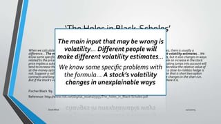
StochasticVolatility Model
StochasticAsset Price and StochasticVolatility
𝑑𝑆𝑡 = 𝜇 𝑡, 𝑆𝑡, 𝑌𝑡 𝑆𝑡 𝑑𝑡 + 𝜎 𝑡, 𝑆𝑡, 𝑌𝑡 𝑆𝑡 𝑑𝐵𝑡
𝑑𝑌𝑡 = 𝑎 𝑡, 𝑆𝑡, 𝑌𝑡 𝑑𝑡 + 𝑏 𝑡, 𝑆𝑡, 𝑌𝑡 𝑑𝑊𝑡
𝑊𝑡 = 𝜌𝐵𝑡 + 1 − 𝜌2 𝑍𝑡, 𝜌 ∈ [−1,1]
Market is incomplete as there is one traded asset and two driving Brownian
MotionsW and B.We can hedge randomness of asset but what about
volatility? No unique risk free measure Q!!!
Heston took 𝜌 ≠ 0, 𝜇 𝑡, 𝑆𝑡, 𝑌𝑡 = 𝜇, 𝜎 𝑡, 𝑆𝑡, 𝑌𝑡 = 𝑌 and volatility follows CIR
process
𝑑𝑆𝑡 = 𝜇𝑆𝑡 𝑑𝑡 + 𝑌𝑡 𝑆𝑡 𝑑𝐵𝑡
𝑑𝑌𝑡 = 𝜅 𝑄 𝛼 𝑄 − 𝑌𝑡 𝑑𝑡 + 𝜈 𝑌𝑡 𝑑𝑊𝑡
Feller condition for Yt > 0, 2𝜅 𝑄 𝛼 𝑄 > 𝜈2

Heston StochasticVolatility Model (Closed
Form)
 To make markets complete, we introduce a second traded asset (e.g. variance swap) 𝑂𝑡 = 𝑢 𝑡, 𝑆𝑡, 𝑌𝑡 hold
∆2 units of it and perform Vega Hedging.
 We proceed in the same way as Black Scholes derivation and create a portfolio
𝑊 = 𝑉 − ∆1 𝑆 − ∆2 𝑂
And to obtain risk neutrality we remove 𝑑𝐵 the risk and 𝑑𝑊 risk, we get
∆1=
𝜕𝑉
𝜕𝑆
−
𝜕𝑢
𝜕𝑆
∆2
𝜕𝑢
𝜕𝑌
∆2=
𝜕𝑉
𝜕𝑌
= 𝑣𝑒𝑔𝑎
𝑑𝑊 = 𝑟 𝑉 − ∆1 𝑆 − ∆2 𝑢 𝑑𝑡
 Fundamental PDE for Heston
1
2
𝑌𝑆2
𝜕2
𝑉
𝜕𝑆2
+ 𝜌𝜈𝑌𝑆
𝜕2
𝑉
𝜕𝑆𝜕𝑌
+
1
2
𝜈2
𝑌
𝜕2
𝑉
𝜕𝑌2
+ 𝑟𝑆
𝜕𝑉
𝜕𝑆
+ 𝜙(𝑆, 𝑉, 𝑡)
𝜕𝑉
𝜕𝑌
− 𝑟𝑉 +
𝜕𝑉
𝜕𝑡
= 0

Risk Neutral to RealWorldTransformation
We have two premiums under the physical measure in the Heston Model
Equity Risk Premium since investors are adverse to negative movements in equity prices.
Volatility Risk Premium since they are adverse to positive movements in volatility.
Equity premium is compensation for risk in 𝑑𝑊𝑡 𝑎𝑛𝑑 𝑑𝐵𝑡. In Heston, these compensations
are proportional to 𝜆′
𝑌 and 𝜆 𝑌 per unit of 𝑑𝑊𝑡 𝑎𝑛𝑑 𝑑𝐵𝑡
𝐸𝑞𝑢𝑖𝑡𝑦 𝑃𝑟𝑒𝑚𝑖𝑢𝑚 = 𝛾𝑆 = 𝜆′
1 − 𝜌2 + 𝜆𝜌
Risk premium for stochastic volatility
𝜙 𝑆, 𝑉, 𝑡 = 𝜅 𝑄 𝛼 𝑄 − 𝑌𝑡 , 𝜅 𝑄 = 𝜅 𝑃 + 𝜆𝜈 , 𝛼 𝑄 =
𝛼 𝑃
1 + 𝜆𝜈
=
𝛼 𝑃 𝜅 𝑃
𝜅 𝑄
𝑉𝑜𝑙𝑎𝑡𝑖𝑙𝑖𝑡𝑦 𝑃𝑟𝑒𝑚𝑖𝑢𝑚 = 𝛾 𝑉 = 𝜆𝜈, 𝛾 𝑉 < 0 (𝜆 < 0)

Summary of RN and RW Heston Model
 Risk neutral dynamics in Heston Model
𝑑𝑆𝑡 = (𝑟 − 𝑞)𝑆𝑡 𝑑𝑡 + 𝑌𝑡 𝑆𝑡 𝑑𝐵𝑡
𝑑𝑌𝑡 = 𝜅 𝑄 𝛼 𝑄 − 𝑌𝑡 𝑑𝑡 + 𝜈 𝑌𝑡 𝑑𝑊𝑡
𝑑𝐵𝑡 𝑑𝑊𝑡 = 𝜌
 Real world dynamics in Heston Model
𝑑𝑆𝑡 = 𝑟 − 𝑞 + 𝛾𝑆 𝑌𝑡 𝑆𝑡 𝑑𝑡 + 𝑌𝑡 𝑆𝑡 𝑑𝐵𝑡
𝑑𝑌𝑡 = 𝜅 𝑃 𝛼 𝑃 − 𝑌𝑡 𝑑𝑡 + 𝜈 𝑌𝑡 𝑑𝑊𝑡
𝑑𝐵𝑡 𝑑𝑊𝑡 = 𝜌
𝜅 𝑃 = 𝜅 𝑄 − 𝛾 𝑉,
𝜅 𝑃
𝜅 𝑄
=
𝛼 𝑄
𝛼 𝑃
 Risk neutral dynamics has lower mean reversion but higher long-run volatility
𝛾𝑆 > 0, 𝛾 𝑉 < 0 ⇒ 𝜅 𝑄 < 𝜅 𝑃 ⇒ 𝛼 𝑄 > 𝛼 𝑃

Heston Stochastic Model Implementation
Further simplify by introducing 𝑥 = ln 𝑆 because then the coefficients do not contain price
of the underlying. Heston solved the PDE using Characteristic Functions.
Monte CarloApproach (Euler Discretization)
-Volatility and price path are discretized using constant ∆𝑡.
- Can lead to discretization errors
𝑌𝑖+1 = 𝑌𝑖 + 𝜅 𝛼 − 𝑌𝑖
+
𝛿𝑡 + 𝛽 𝑌𝑖
+
𝛿𝑊𝑖+1
𝑋𝑖+1 = 𝑋𝑖 exp 𝜇 −
1
2
𝑌𝑖
+
𝛿𝑡 + 𝑌𝑖
+
𝛿𝑡𝛿𝐵𝑖+1
𝑋𝑡 = ln 𝑆 𝑇 , 𝑧+
= max(𝑧, 0)

Heston StochasticVolatility Model
Parameters
Heston Parameters
• 𝜌 affects the skewness of the distribution (leverage affect)
• 𝜌 > 0 ⇒spread the right tail and squeeze left tail of asset return dist.
• 𝜌 < 0 ⇒spread the left tail and squeeze right tail of asset return dist.
• 𝛽 affects the kurtosis of the distribution, high 𝛽 means heavy tails
• 𝜅 affects the degree of “volatility clustering”
• 𝛼 is the long run variance
• 𝑌0 is the initial variance and it affects the height of the smile curve

Calibration of Heston Model
Minimize the least squared error between market price for a given range of expiries and
strikes and the model price.
Local Optimizer like Levenberg-Marquardt
• Depends on the selection of seed values (initial guess)
• Determines optimal direction of search
• Possibility of finding local minima
• Only searches small amount of the search space
Find best fit to ATM volatilities because they are the most liquid.
Global optimization approaches better but takes too long.

Pros and Cons of Heston Model
Advantages of Heston SVM
• Non Lognormal probability
distribution in price dynamics
• Volatility is mean reverting
• Takes into account leverage
effect between equity returns
and volatility
 Disadvantages of Heston SVM
− Calibration is often difficult due
to number of parameters to fit
− Expensive to do global
optimization.
− Prices are sensitive to
parameters

Agenda
 Black Scholes Pricing Model
 Holes in the Black-Scholes Model
 Importance ofVolatility Estimation
 Stylized Facts aboutVolatility
 Volatility Models
• LocalVolatility Models
• StochasticVolatility Models
 Stochastic Volatility Jump Diffusion

StochasticVolatility Jump Diffusion
The stochastic volatility model captures some stylized facts:
• Volatility clustering
• Mean Reversion
• Heavier tails
Fails to capture random fluctuations (for e.g. shock in the market causing crash)
𝑑𝑆𝑡 = 𝜇𝑆𝑡 𝑑𝑡 + 𝑌𝑡 𝑑𝑊𝑡 + 𝐽 − 1 dNt
𝑑𝑌𝑡 = 𝜅 𝛼 − 𝑌𝑡 + 𝜈 𝑌𝑡 𝑑𝐵𝑡
𝑑𝑊𝑡 𝑑𝐵𝑡 = 𝜌
𝑃 𝑁 𝑡 = 𝑘 =
𝜆𝑡 𝑘
𝑘!
𝑒−𝜆𝑡
log 𝐽~𝑁(𝑚, 𝜎2
)

References
1. Dupire B, 1994 Pricing with a smile
2. Gyongy I, 1986 Mimicking the One-Dimensional Marginal Distribution of Processes Having and
Ito Differential
3. Heston SL, 1993 A closed-form solution for options with stochastic volatility with applications to
bond and currency options
4. Hagan P, Kumar D, Lesniewski A and DWoodward 2002, Managing Smile Risk
5. Monoyios, Michael 2007 StochasticVolatility , University of Oxford
6. Ruf, Johannes 2015 Local and StochasticVolatility, Oxford-Man Institute of Quantitative
Finance

Local and Stochastic volatility

More Related Content

What's hot

Viewers also liked

Similar to Local and Stochastic volatility

Recently uploaded

Local and Stochastic volatility