Instrument characteristics

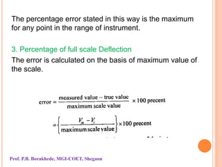
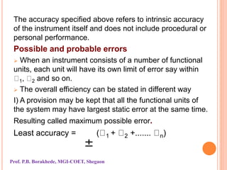
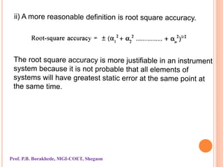
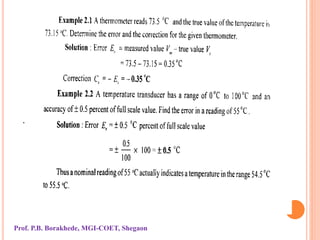
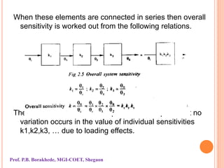
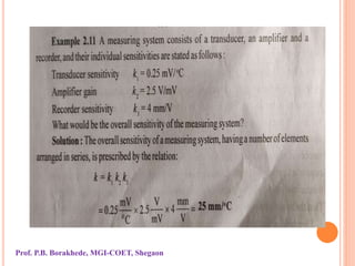
MEASUREMENT SYSTEMS
Unit No 2
Instrument Characteristics

INTRODUCTION
 In this unit we would discuss how well an instrument
performs its various functions.
 The instrument performance is described by means of
quantitative qualities which are referred to as
characteristics ir static and dynamic.
 The static characteristics pertain to a system where
quantities to be measured are constant or vary slow with
time.
 Dynamic characteristics are quantities to be measured
are varying speedely with time.
Prof. P.B. Borakhede, MGI-COET, Shegaon

STATIC CHARACTERISTICS
1. Range and Span
a) Range
 The region between the limits within which an
instrument is designed to operate for measuring,
indicating or recording a physical quantity is called
range of instrument.
 The range is expressed by stating the lower and upper
values.
b) Span
 Span represents algebric differences between the
upper and lower range values of the instrument.

 For example
Range -10ᵒ C to 80ᵒ C; Span 90ᵒ C
Range 5 bar to 100 bar Span 95 bar
Range 0 to 75 volt; Span 75
2. Accuracy, Error, Correction
 No instrument gives an exact value of what is being
measured.
 There is always some uncertaintity in the measured
value.
 This uncertainty is expressed in terms of accuracy
and error.

a) Accuracy
 Accuracy of an indicated ( measured) value can be
defined as conformity with or closeness to an
accepted standard value ( true value).
 Accuracy of the measured signal depends upon:
1. Intrinsic accuracy of the instrument itself.
2. Variation of the signal being measured.
3. Accuracy of the observer
4. Whether or not the quantity is being impressed
upon the instrument.
 For example: The accuracy of a micrometer depends
upon factors like errors in screw, anvil shape,
temperature difference and applied torque variations
etc.

b) Error
 In general, the result of any measurement differs
somewhat from the true value of quantity being
measured.
 The difference between measured value (Vm) and true
value (Vt) of the quantity represents the static or
absolute error of measurement (Es).
 Es = Vm - Vt
 Error can be positive or negative. For positive static
errors the instrument reads high and for negative
static error instrument reads low.
 Accuracy is being measured in terms of errors.

C) Correction
 From experiment point of view correction is more
important than static error.
 The static correction is defined as difference between
true value and measured value of a quantity.
 Cs =Vt - Vm
 The correction of an instrument reading is of same
magnitude as the error but opposite in signal Cs =
-Es

Error specification or representation
1. Point accuracy
The accuracy of instrument is stated for one or more
points in its range.
For example: A given thermometer may be stated to read
within 0.5°C between 100°C and 200°C. Likewise a scale
of length may be read within 0.025 cm.
2. Percentage of true value or Relative Error
The absolute error of measurement is expressed as a
percentage of true value of unknown quantity.

The percentage error stated in this way is the maximum
for any point in the range of instrument.
3. Percentage of full scale Deflection
The error is calculated on the basis of maximum value of
the scale.

The accuracy specified above refers to intrinsic accuracy
of the instrument itself and does not include procedural or
personal performance.
Possible and probable errors
 When an instrument consists of a number of functional
units, each unit will have its own limit of error say within
1, 2 and so on.
 The overall efficiency can be stated in different way
I) A provision may be kept that all the functional units of
the system may have largest static error at the same time.
Resulting called maximum possible error.
Least accuracy = ( 1 + 2 +....... n)

Calibration
 The magnitude of error and correction to be applied
is determined by making a periodic comparison of
the instrument with standards which are known to
be constant.
 The entire procedure of checking, making or
adjusting a scale so that readings of an instrument
or measurement system confirm to an accepted
standard is called calibration.
 The graphical representation of calibration record is
called calibration curve.

The following points needs consideration while calibrating
an instrument
1. Calibration of instrument is carried out with the
instrument in the same position (upright, horizontal etc)
and subjected to same temperature and other
environmental conditions under which it is to operate
while in service.
2. The instrument is calibrated with values of measurand
impressed both in increasing and decreasing order.
The results are then expressed graphically; output is
plotted as ordinate and input or measurand as the
abscissa.
3. Output readings for a series impressed values going up
the scale may not agree with the output readings for
the same input values going down.

Calibration Curve
 In a typical calibration
Curve, ABC represents readings obtained while
ascending the scale. DEF
represents readings during
descend, KLM represents the
median and is commonly
accepted as calibration curve.
 The term median refers to the mean of a series of up
and down readings.

Correction Curve
 The indicated values are
plotted abscissa and ordinate
represents the variation of
Median from the true values.
 A faired curve through
Experimental points then represents as correction curve.
 This curve shows rapid visual assessment of accuracy of
instrument.
 A properly prepared calibration curve gives information
about the absolute static error, extent of instruments
linearity or conformity, and hysteresis and repeatability of
the instrument.

 Hysteresis and Dead Zone
Hysteresis
Hysteresis is the maximum difference for the same
measured quantity( input signal) between the upscale
from zero to maximum and downscale readings from
maximum to zero during a full range transverse in each
direction.
Maximum difference is frequently specified as a
percentage of full scale.
Hysteresis causes because of mechanical friction, slack
motion in bearings and gears, elastic deformation,
magnetic and thermal effects.
Hysteresis also occurs in electronic system due to
heating and cooling effects which occur differentially
under conditions of rising and falling inputs.

Dead Zone
 Dead zone is the largest range through which an input
signal can be varied without imitating any response from
the indicating instrument.
It is largest change of input quantity for which instrument
does not indicate output.
Friction or play is the cause of dead zone.
 Drift
It is an undesired gradual departure of the instrument
output over a period of time that is not related to changes
in input.
An instrument said to have no drift if it reproduces same
readings at different times for same variation in
measured variables.

The following factors may lead to drift in an instrument:
a) Wear and tear at the mating parts
b) Mechanical vibrations
c) Contamination of primary sensing elements
d) Development of high mechanical stresses in some
parts.
e) Temperature changes, stray electric and magnetic
fields.
Examples:
1. Drift occurs in thermocouples and resistance
thermometers due to contamination of the metal and
a change in its metallurgical structure.

 Sensitivity
 Sensitivity of an instrument is ratio of the magnitude of
the response( output signal) to the magnitude of the
quantity being measured( input signal).
 Sensitivity (K) = Change in output signal/ Change in
input signal.
 Sensitivity is represented by the slope of the calibration
curve the sensitivity is constant.
 With a linear calibration curve, the sensitivity is constant.
 If the calibration curve is non linear the static sensitivity
is not constant.

 Sensitivity has a wide range of units and these depend
upon the instrument being investigated.
 Sensitivity of an instrument system is usually required to
be as high as possible because then it becomes easier
to take measurement( read the output).
 Let different elements comprising a measurement
system have static sensitivities of k1, k2, k3… etc.

When these elements are connected in series then overall
sensitivity is worked out from the following relations.
The above relation is based upon the assumption that no
variation occurs in the value of individual sensitivities
k1,k2,k3, … due to loading effects.

Threshold and Resolution
The smallest increment of quantity being measured
which can be detected with certainty by an instrument
represents the threshold and resolution of the
instrument.
Threshold
When the input signal to an instrument is gradually
increased from zero, there will be some minimum value
input before which the instrument will not detect any
output change.
This minimum value is called threshold of the instrument.
Threshold defines as the minimum value of input which
is necessary to cause detectable change from zero
output.
Threshold may cause by backlash or internal noise.

Resolution
 When the input signal is increased from non zero value,
it is observed that instrument output does not change
until a certain input increment is exceeded. This
increment is called as resolution.
 Resolution is defines the smallest change of input for
which there will be a change in output.
 With analog instruments, resolution is determined by
the ability of the observer to judge the position of a
pointer scale. Eg the level of mercury in a glass tube.
 Threshold and resolution may be expressed as an
actual value or as a fraction or percentage of full scale.

Precision and Repeatability
Precision
Accuracy refers to closeness to true value of the quantity
under measurement while precision refers to the ability
of instrument to reproduce its readings over and over
again for a constant input signal.
Precision is also called as repeatability.
It is defined as the closeness of agreement between
independent test results, obtained with the same
method, on the same test material, in the same
laboratory, by the same operator and using the same
equipment within short interval of time.
Difference between accuracy and precision is shown by
following example.

The arrangement may be though to correspond to the
game of darts where a person is asked to strike a target
represented by centre circle.
The centre circle represents true value, and the result
achieved by the striker has been indicated by mark *
Reproducibility
 Reproducibility is the closeness between measurements
of the same quantity when the individual measurements
are made under different conditions such as
 At different location
 By different operators
 Under different conditions of instrument use
 With different measuring instruments
 Over long time periods.

Linearity
 The working range of most of the instruments provides a
linear relationship between output and input.
 This aspect tends to facilitate more accurate data
reduction.
 Linearity is defined as the ability to reproduce the input
characteristics symmetrically, and this can be expressed
by the straight line equation.
 It can be expressed equation y = mx+c.
 Where y it output, x is input, m is slope and c is
intercept.
 The closeness of the calibration curve to a specified
straight line linearity of the instrument.

 Any departure from the straight line relationship is non
linearity.
 The non linearity may be due to
 Non linear elements in the mechanical device
 Mechanical hysteresis
 Viscous flow or creep
 Elastic after effects in the mechanical system.

DYNAMIC CHARACTERISTICS
 When the instruments are required to measure an input
which is varying with time, the dynamic or transient
behavior of the instrument becomes as important.
 Some dynamic terms are as follows:
Speed of Response and Measuring Lag
Speed of response:
In measuring instruments the speed of response or
responsiveness is defined as the rapidity with which an
instrument responds to a change in value of the quantity
being measured.

Measuring Lag
Measuring lag refers to retardation or delay in the
response of an instrument to a change in the input
signal. The lag is caused by conditions such as
capacitance, inertia, or resistance.
Measuring lags are of two types:
a) Retardation type:
In this case the response of the measurement system
begins immediately after the change in measured
quantity has occurred.
b)Time delay Type:
In this case the response of the measurement system
begins after a dead time after the application of the
input.

Fidelity and Dynamic Error
Fidelity
Fidelity of the instrumentation system is defined as the
degree of closeness with which the system indicates or
records signal which is impressed upon it.
It refers the ability of the system to reproduce the output
in the same form as the input.
If the input is a sine of wave then for 100 percent fidelity,
the output should also be a sine wave.
Dynamic Error
The difference between the indicated quantity and the
true value of the time varying quantity is the dynamic
error. Here static error is assumed to be zero.

Dead Time and Dead Zone
Dead Time
 Dead time is defined as the time required for an
instrument to begin to respond to a change in the
measured quantity.
It represents the time before the instrument begins to
respond after the measured quantity has been altered.
Dead Zone
Dead zone defines the largest change of the
measurand to which the instrument does not respond.
Dead zone is the result of friction, backlash or
hysteresis in the instrument.

 Overshoot:
 Because of mass and inertia, a moving part ie, the pointer
of the instruments does not immediately come to rest in
the final deflected position.
The pointer goes beyond the steady state ie it overshoots.
The overshoot is defined as the maximum amount by
which the pointer moves beyond the steady state.

Standard Test inputs
 The dynamic performance of both measuring and
control systems is determined by applying some known
and predetermined input signals to its primary sensing
element and then studying behavior of the output signal.
 Most common standard inputs used for dynamic
analysis have been illustrated in figure.
1. Step Function
which is sudden change from one steady value to
another.
The step input is mathematically represented by
relationship
ᶿi = 0 at t<0
ᶿi= ᶿo at t>0

Where ᶿo is a constant value of input signal ᶿi .
2. Ramp or Linear function
In this input varies linearly with time. The ramp input is
mathematically represented as:
ᶿi = 0 at t<0
ᶿi= Ωt at t>0
Where Ω is slope of input versus time relationship.
3. Sinusoidal or sine wave function
Here input has a cyclic variation; the input varies
sinusoidally with a constant maximum amplitude.
It is represented as ᶿi = A sinωt where
A is amplitude and ω is the frequency in rad/sec.

A general measurement system can be mathematically
described by the following differential equation

The time factor in the input or driving function may
correspond to step input, ramp input, sinusoidal input or
any combination of these.
The order of the measurement system is generally
classified by the value of the power of n.

Zero, First, and second order system
1. Zero Order System
Consider an ideal measuring system ie system whose
output is directly proportional to input; no matter how
the input varies.
The output is a faithful reproduction of input without any
distortion or time lag.
The mathematical equation relating output to input is
ᶿi= K ᶿo
Where K is sensitivity of the system.
This equation of the zero order system and its value can
be obtained through the process of calibration.
Block diagram represents zero order system

Examples of zero order system are
Mechanical levers, amplifiers and potentiometer which
gives output as input.
2. First order System
The behavior of a first order system is represented by a
first order differential equation of the form

Examples of first order system
1. Temperature measurement by mercury-in- glass
thermometers, thermocouples and thermistors.
2. Build up air pressure bellows
3. Network of resistance capacitance
4. Velocity of a free failing mass.

3. Second Order System

Examples of second order system
1. Spring mass system employed for acceleration
and force measurement
2. Piezo electric pick ups
3. UV galvanometer
4. Pen control system on XY plotters.

IMPORTANT QUESTIONS
 Define Following terms:
i) Accuracy ii) precision iii) Range and span iv) sensitivity
v) Measuring Lag vi) Overshoot.
 Define following terms:
i) Dead time ii) Dead zone iii) Hysteresis iv) Resolution v)
Drift vi) Speed of Response vii) Fidelity.
 Obtain an expression for zero order, first order and
second order system.
 What is scale readability? What are the factors on
which readability depends?
 Define dynamic response of a system and distinguish
between steady stare and transient response.
 Distinguish between precision and accuracy.

Instrument characteristics

More Related Content

What's hot

Similar to Instrument characteristics

More from Prashant Borakhede

Recently uploaded

Instrument characteristics