This document provides a comprehensive list of important formulas for subjects related to commerce, management, economics, finance, accounting, and statistics that are relevant for UGC NET exams. It includes over 50 formulas organized into sections on economics, macroeconomics, accounting, finance, statistics, and bonds valuation. The formulas cover concepts like GDP, costs, revenues, profits, ratios, probabilities, and present value. Having these formulas in one place will help exam preparation by allowing aspirants to efficiently review essential quantitative concepts and calculations.
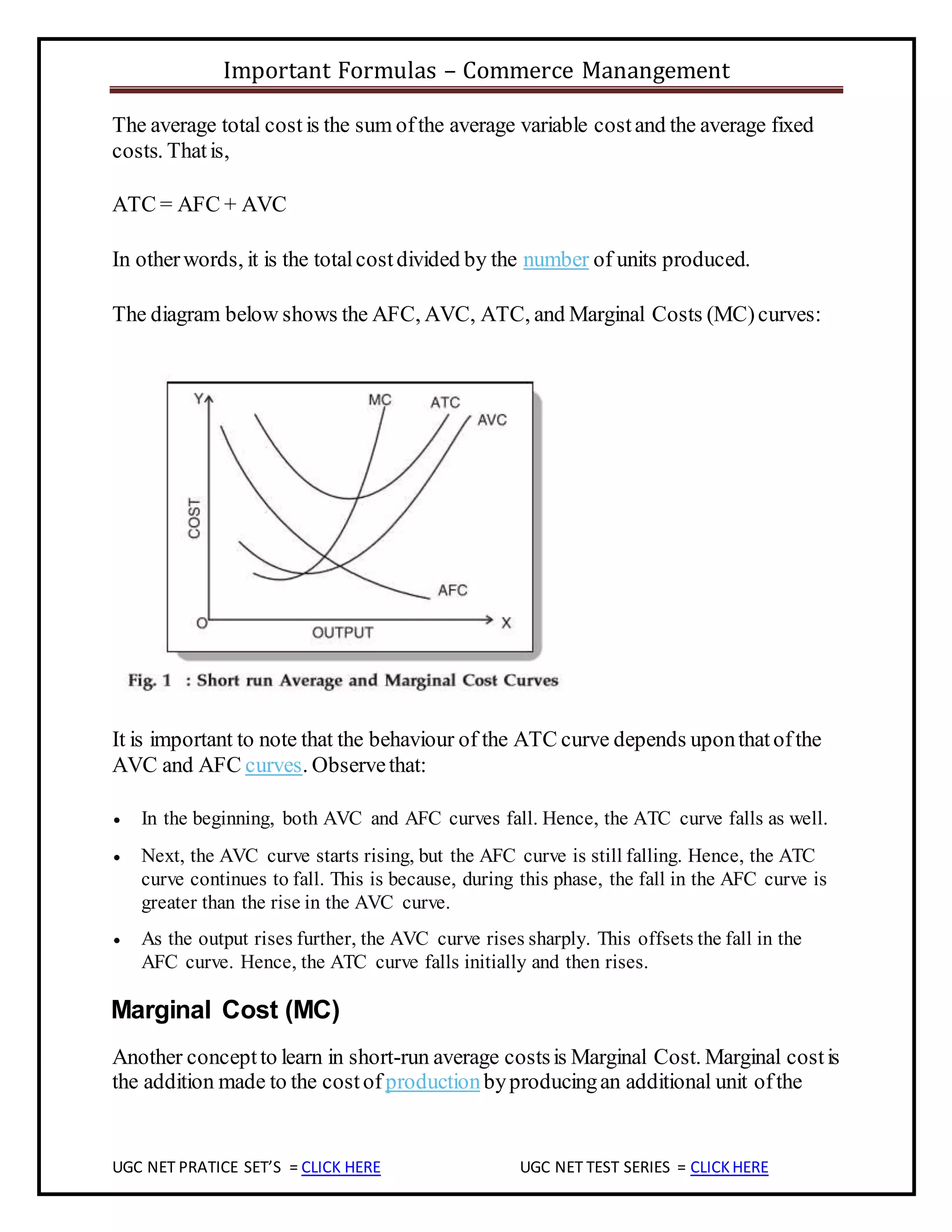
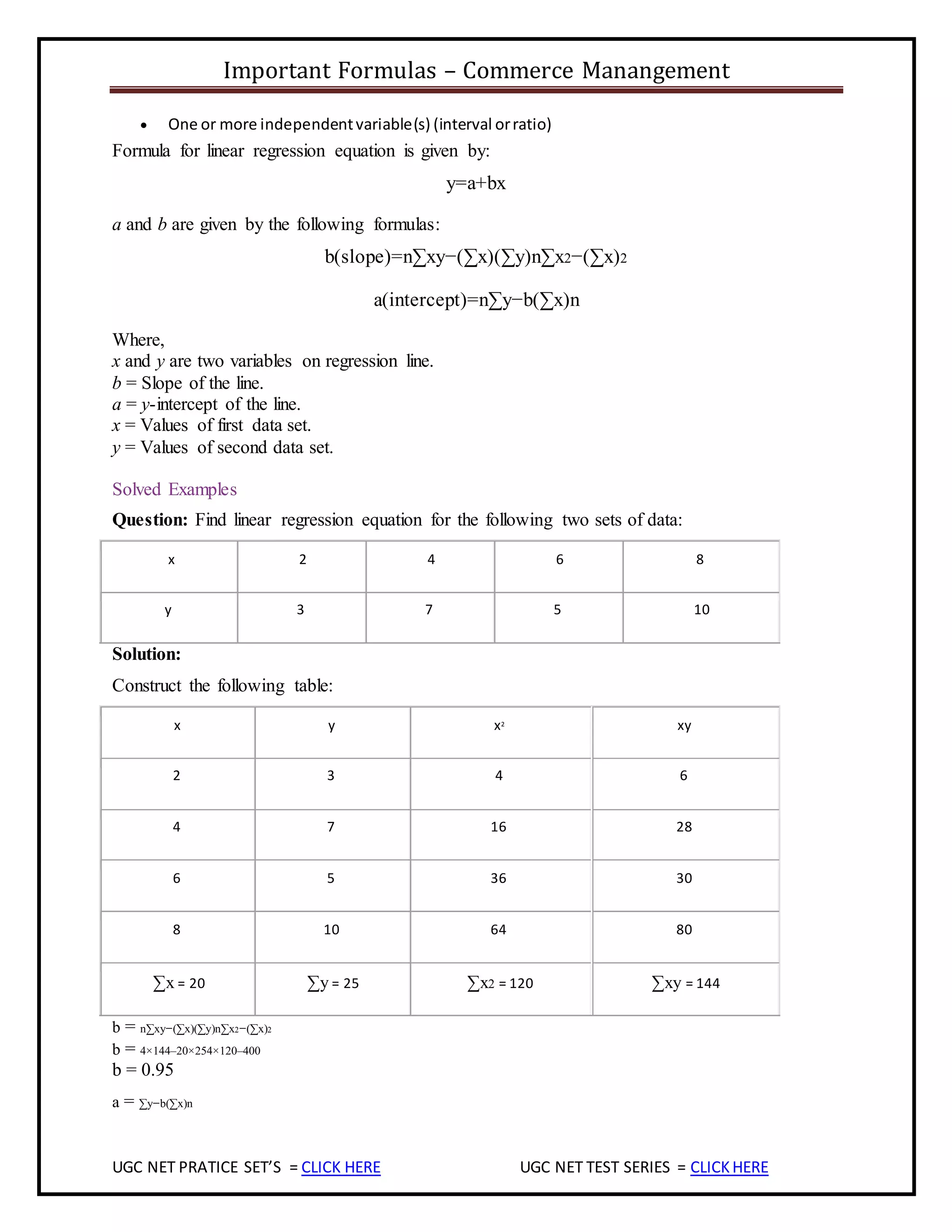
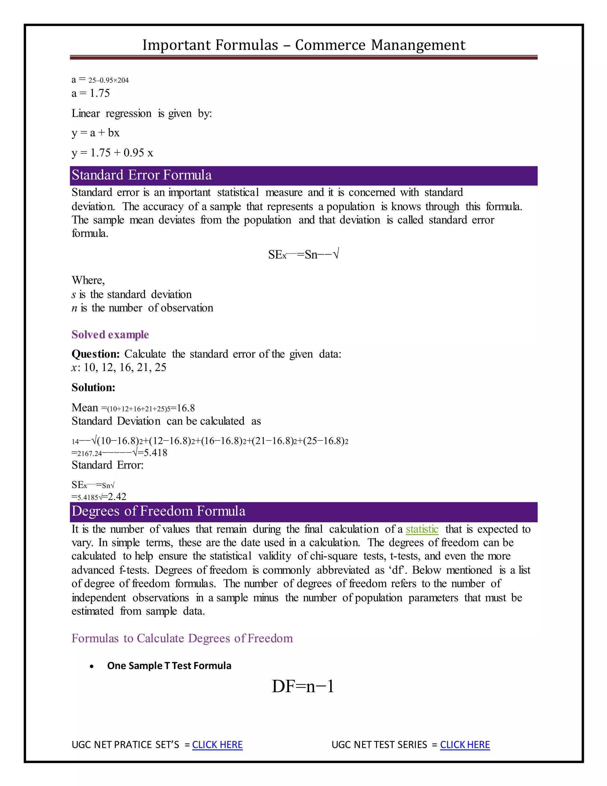
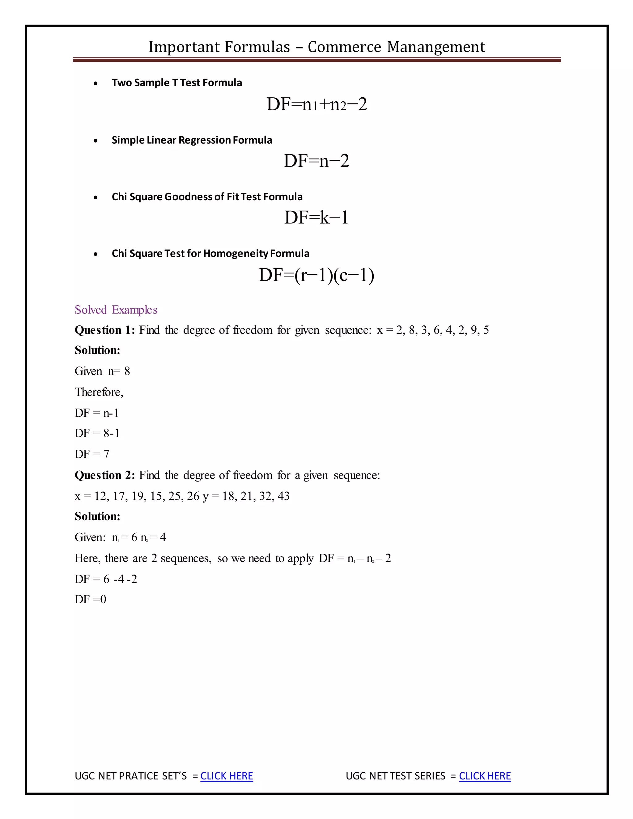
![Important Formulas – Commerce Manangement
UGC NET PRATICE SET’S = CLICK HERE UGC NET TEST SERIES = CLICKHERE
= Current Assets / Current Liabilities
1. Quick/Acid Test ratio:
= (Current Assets – Inventory) / Current Liabilities
1. Average Collection Period:
= Average Accounts Receivable /(Annual Sales/360)
1. PROFITABILITY RATIOS:
Profit Margin (on sales):
= [Net Income / Sales] X 100
Return on Assets:
= [Net Income / Total Assets] X 100
Return on equity:
= [Net Income/Common Equity]
6. ASSET MANAGEMENT RATIOS
Inventory Turnover:
= Sales / inventories
Total Assets Turnover:
= Sales / Total Assets
1. DEBT (OR CAPITAL STRUCTURE) RATIOS:
Debt-Assets:
= Total Debt / Total Assets
Debt-Equity:
= Total Debt / Total Equity
Times-Interest-Earned:
= EBIT / Interest Charges
1. Market Value Ratios:
Price Earning Ratio:
= Market Price per share / *Earnings per share
Market /Book Ratio:
= Market Price per share / Book Value per share
*Earning Per Share (EPS):
= Net Income / Average Number of Common Shares Outstanding](https://image.slidesharecdn.com/importantformulesforugcnetcommercemanagementmostimportantdownloadpdfquickrevision-191229104843/75/Important-formules-for-ugc-net-commerce-management-most-important-download-pdf-quick-revision-8-2048.jpg)
![Important Formulas – Commerce Manangement
UGC NET PRATICE SET’S = CLICK HERE UGC NET TEST SERIES = CLICKHERE
1. Estimated current assets for the next year
= [Current assets for the current year/Current sales] x Estimated sales for the next year
1. Expected Estimated retained earnings
= estimated sales x profit margin x plowback ratio
1. Estimated discretionary financing
= estimated total assets – estimated total liabilities –estimated total equity
1. G (Desired Growth Rate)
= return on equity x (1- pay out ratio)
1. Interest Rates for Discounting Calculations
• Nominal (or APR) Interest Rate = i nom
• Periodic Interest Rate = i per
It is defined as
iper = ( i nominal Interest rate) / m
Where
m = no. of times compounding takes place in 1 year i.e.
If semi-annual compounding then m = 2
• Effective Interest Rate = i eff
i eff = [1 + ( i nom / m )]m – 1
1. Calculating the NPV of the Café Business for 1st Year:
NPV = Net Present Value (taking Investment outflows into account)
NPV = −Initial Investment + Sum of Net Cash Flows from Each Future Year.
NPV = − Io +PV (CF1) + PV (CF2) + PV (CF3) + PV (CF4) + ...+ ∞
1. Annual Compounding (at end of every year):
FV = CCF (1 + i) n – 1
Annual Compounding (at end of every year)
PV =FV / (1 + i ) n . n = life of Annuity in number of years](https://image.slidesharecdn.com/importantformulesforugcnetcommercemanagementmostimportantdownloadpdfquickrevision-191229104843/75/Important-formules-for-ugc-net-commerce-management-most-important-download-pdf-quick-revision-10-2048.jpg)
![Important Formulas – Commerce Manangement
UGC NET PRATICE SET’S = CLICK HERE UGC NET TEST SERIES = CLICKHERE
1. Multiple Compounding:
Future Value of annuity =CCF (constant cash flow)*(1+ (i/m) m*n-1/i/n
Multiple Compounding:
PV =FV / [1 + (i/m)] mxn
1. Future value of perpetuity:
=constant cash flow/interest rate
1. Future value by using annuity formula
FV =CCF [(1+i) n - 1]/ i
1. Return on Investments:
ROI= (ΣCF/n)/ IO
1. Net Present Value (NPV):
NPV= -IO+ΣCFt/ (1+i) t
Detail
NPV = -Io + CFt / (1+i)t = -Io + CF1/(1+i) + CF2/(1+i) ^2 + CF` /(1+i)^3 +..
-IO= Initial cash outflow
i=discount /interest rate
t=year in which the cash flow takes place
1. Probability Index:
PI = [Σ CFt / (1+ i) t ]/ IO
1. Internal Rate Of Return(IRR) Equation:
NPV= -IO +CF1/ (1+IRR) + CF2/ (1+IRR) ^2......
1. Internal Rate of Return or IRR:
The formula is similar to NPV](https://image.slidesharecdn.com/importantformulesforugcnetcommercemanagementmostimportantdownloadpdfquickrevision-191229104843/75/Important-formules-for-ugc-net-commerce-management-most-important-download-pdf-quick-revision-11-2048.jpg)
![Important Formulas – Commerce Manangement
UGC NET PRATICE SET’S = CLICK HERE UGC NET TEST SERIES = CLICKHERE
NPV = 0 = -Io + CFt / (1+IRR)t = -Io + CF1/(1+IRR) + CF2/(1+IRR) ^2 + ..
1. Modified IRR (MIRR):
(1+MIRR) n = Future Value of All Cash Inflows….
Present Value of All Cash Outflows
(1+MIRR) n = CF in * (1+k) n-t
CF out / (1+k) t
1. Equivalent Annual Annuity Approach:
EAA FACTOR = (1+ i)^ n / [(1+i)^ n -1]
Where n = life of project & i=discount rate
BONDS’ VALUATION
The relationship between present value and net present value
1. NPV = -Io + PV
1. Present Value formula for the bond:
n
PV= Σ CFt / (1+rD)t =CF1/(1+rD)+CFn/(1+rD)2 +..+CFn/ (1+rD) n +PAR/ (1+rD) ^n
t =1
In this formula
PV = Intrinsic Value of Bond or Fair Price (in rupees) paid to invest in the bond. It is the
Expected or Theoretical Price and NOT the actual Market Price.
rD = it is very important term which you should understand it care fully. It is
Bondholder’s (or
Investor’s) Required Rate of Return for investing in Bond (Debt).As conservative you
can choose
minimum interest rate. It is derived from Macroeconomic or Market Interest Rate.
Different from the Coupon Rate!
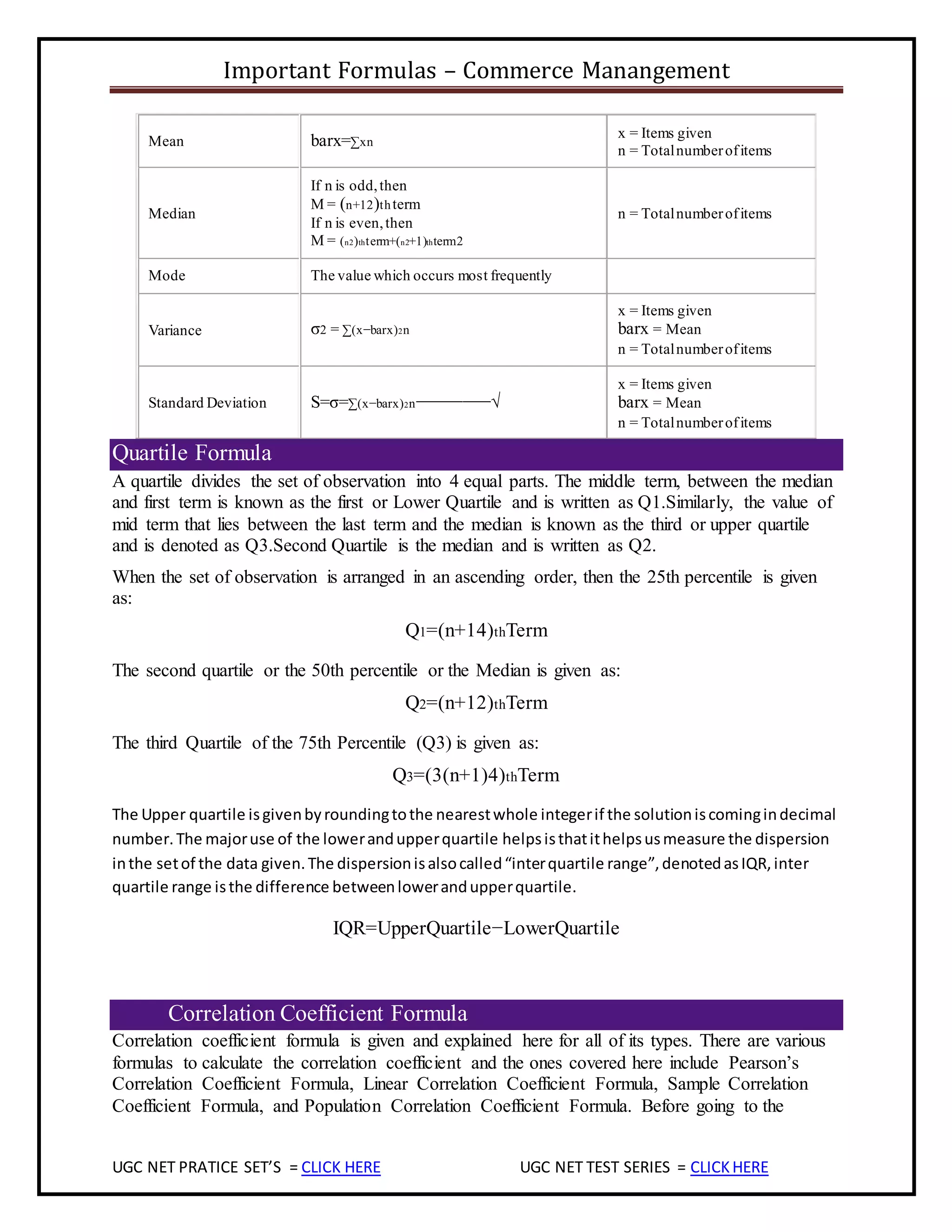
STATISTICS FORMULS –
The important statistics formulas are listed in the chart below:](https://image.slidesharecdn.com/importantformulesforugcnetcommercemanagementmostimportantdownloadpdfquickrevision-191229104843/75/Important-formules-for-ugc-net-commerce-management-most-important-download-pdf-quick-revision-12-2048.jpg)
![Important Formulas – Commerce Manangement
UGC NET PRATICE SET’S = CLICK HERE UGC NET TEST SERIES = CLICKHERE
Types of Correlation Coefficient Formula
There are several types of correlation coefficient formulas. But, one of the most commonly used
formulas in statistics is Pearson’s Correlation Coefficient Formula. The formulas for all the
correlation coefficient are discussed below.
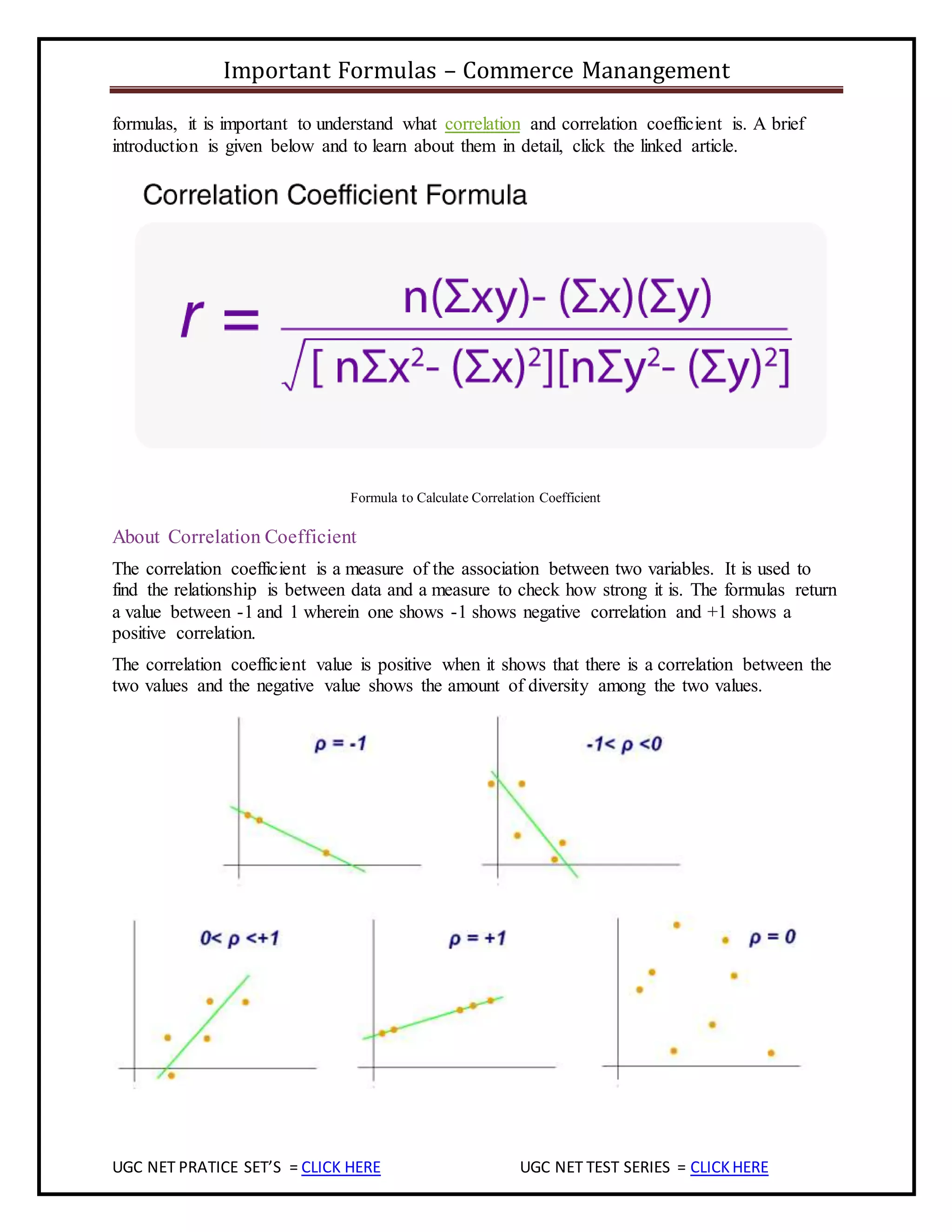
Pearson’s Correlation Coefficient Formula
Also known as bivariate correlation, the Pearson’s correlation coefficient formula is the most
widely used correlation method among all the sciences. The correlation coefficient is denoted by
“r”.
To find r, let us suppose the two variables as x & y, then the correlation coefficient r is calculated
as:
r=n(∑xy)−(∑x)(∑y)[n∑x2−(∑x)2][n∑y2−(∑y)2]−−−−−−−−−−−−−−−−−−−−−−−−−−−√
Notations:
n Quantity ofInformation
Σx Totalof the First Variable Value
Σy Totalof the Second Variable Value
Σxy Sumof the Product of & Second Value
Σx2
Sumof the Squares ofthe First Value
Σy2
Sumof the Squares ofthe Second Value
Linear Correlation Coefficient Formula
The linear correlation coefficient formula is given by the following formula
Sample Correlation Coefficient Formula
rxy=SxySxSy
Here, Sx and Sy are the sample standard deviations, and Sxy is the sample covariance.
Population Correlation Coefficient Formula
ρxy=σxyσxσy
The population correlation coefficient uses σx and σy as the population standard deviations and
σxy as the population covariance.](https://image.slidesharecdn.com/importantformulesforugcnetcommercemanagementmostimportantdownloadpdfquickrevision-191229104843/75/Important-formules-for-ugc-net-commerce-management-most-important-download-pdf-quick-revision-15-2048.jpg)


![CUET MA Psychology Book PDF [Sample]](https://cdn.slidesharecdn.com/ss_thumbnails/cuetmapsysmptm-221017114817-536a1dae-thumbnail.jpg?width=640&height=640&fit=bounds)
![CSIR NET Life Science book.pdf [Sample]](https://cdn.slidesharecdn.com/ss_thumbnails/freesamplecsirnetlifescience1-221017122619-cc591fda-thumbnail.jpg?width=640&height=640&fit=bounds)
![GATE Botany Book PDF [Sample PDF]](https://cdn.slidesharecdn.com/ss_thumbnails/botanysamcp11-221017121855-79fc75de-thumbnail.jpg?width=640&height=640&fit=bounds)
![UGC NET Physical Education Book pdf [ Sample]](https://cdn.slidesharecdn.com/ss_thumbnails/freesampleugcnetphysicaleducation-221017115756-e422cc45-thumbnail.jpg?width=640&height=640&fit=bounds)
![UGC NET Sociology In Hindi book pdf [Sample]](https://cdn.slidesharecdn.com/ss_thumbnails/freesampleugcnetsociologyinhindi1-221017120245-d61d36df-thumbnail.jpg?width=640&height=640&fit=bounds)
![UGC NET Sanskrit Book PDF [Sample]](https://cdn.slidesharecdn.com/ss_thumbnails/ugcsunskritsmp2-221017120832-502d3565-thumbnail.jpg?width=640&height=640&fit=bounds)

![CSIR NET Chemical Science [Chemsirtry] Book PDF [Sample PDF]](https://cdn.slidesharecdn.com/ss_thumbnails/chsnewsample2-221017115228-e79e62c1-thumbnail.jpg?width=640&height=640&fit=bounds)
![CUET MA Economics book .pdf [Sample PDF]](https://cdn.slidesharecdn.com/ss_thumbnails/samplepdfcuetmaeconomics1-221017122155-ae31840f-thumbnail.jpg?width=640&height=640&fit=bounds)
![UGC NET History In Hindi Book PDF [Sample]](https://cdn.slidesharecdn.com/ss_thumbnails/freesampleugcnethistoryinhindi1-221017120604-7857aaeb-thumbnail.jpg?width=640&height=640&fit=bounds)
![UGC NET Environment Science [EVS] Book PDF [Sample]](https://cdn.slidesharecdn.com/ss_thumbnails/freesampleugcnetevs2-221017115418-5f115a15-thumbnail.jpg?width=640&height=640&fit=bounds)
![UGC NET Education [Code-09] Book pdf [Sample PDF]](https://cdn.slidesharecdn.com/ss_thumbnails/freesampleugcneteducation-221017121434-bf8c7ab3-thumbnail.jpg?width=640&height=640&fit=bounds)
![UGC NET Managemnet Book PDF [Sample]](https://cdn.slidesharecdn.com/ss_thumbnails/freesampleugcnetmanagement2-221017114629-7fa5f8c9-thumbnail.jpg?width=640&height=640&fit=bounds)


![UGC NET Computer Science & Application book.pdf [Sample]](https://cdn.slidesharecdn.com/ss_thumbnails/freesampleugcnetcomputerscienceapplication5-221017120357-ff322815-thumbnail.jpg?width=640&height=640&fit=bounds)

![UGC NET Economics Book in Hindi PDF [Sample]](https://cdn.slidesharecdn.com/ss_thumbnails/freesampleugcneteconomics1-221017120002-d97bee62-thumbnail.jpg?width=640&height=640&fit=bounds)


