Principle of microeconomic.pptx

ECON 201: Principles of
Microeconomics
Russell S. Sobel, Ph.D.
Professor of Economics and Entrepreneurship
Baker School of Business
The Citadel

ECON 201: Principles of
Microeconomics
 Chapter 8: Costs and the Supply of
Goods

The Organization of the
Business Firm
 In privately owned firms, owners risk their wealth on
the success of the business. If the firm is successful
and earns profits, these financial gains go to the
owners. Conversely, if the firm suffers losses, the
owners must bear the consequences.
 The property right of owners to the residual income of
the firm plays a very important role: It provides
owners with a strong incentive to organize and operate
their business in a manner that will maximize the value
of their output to consumers while keeping the cost of
producing output low and not wasting resources.

Shirking
 Imperfect monitoring, information, and mis-
aligned incentives are always a problem
confronted by owners with team production that
happens within a business firm.

Test Yourself
 Question: If your new boss asked “how
big of an office do you want?” what
would you answer?
 What are some ways the pay of
managers and employees may be
structured to align the incentives of the
employees with the owners?

Types of Business Firms
Roughly 50% of American’s
own stock either directly or
through their retirement accts.
Advantages &
Disadvantages…
(next slide) 
Firm incentive is
to maximize long-
run (discounted)
net profit/value for
shareholders.

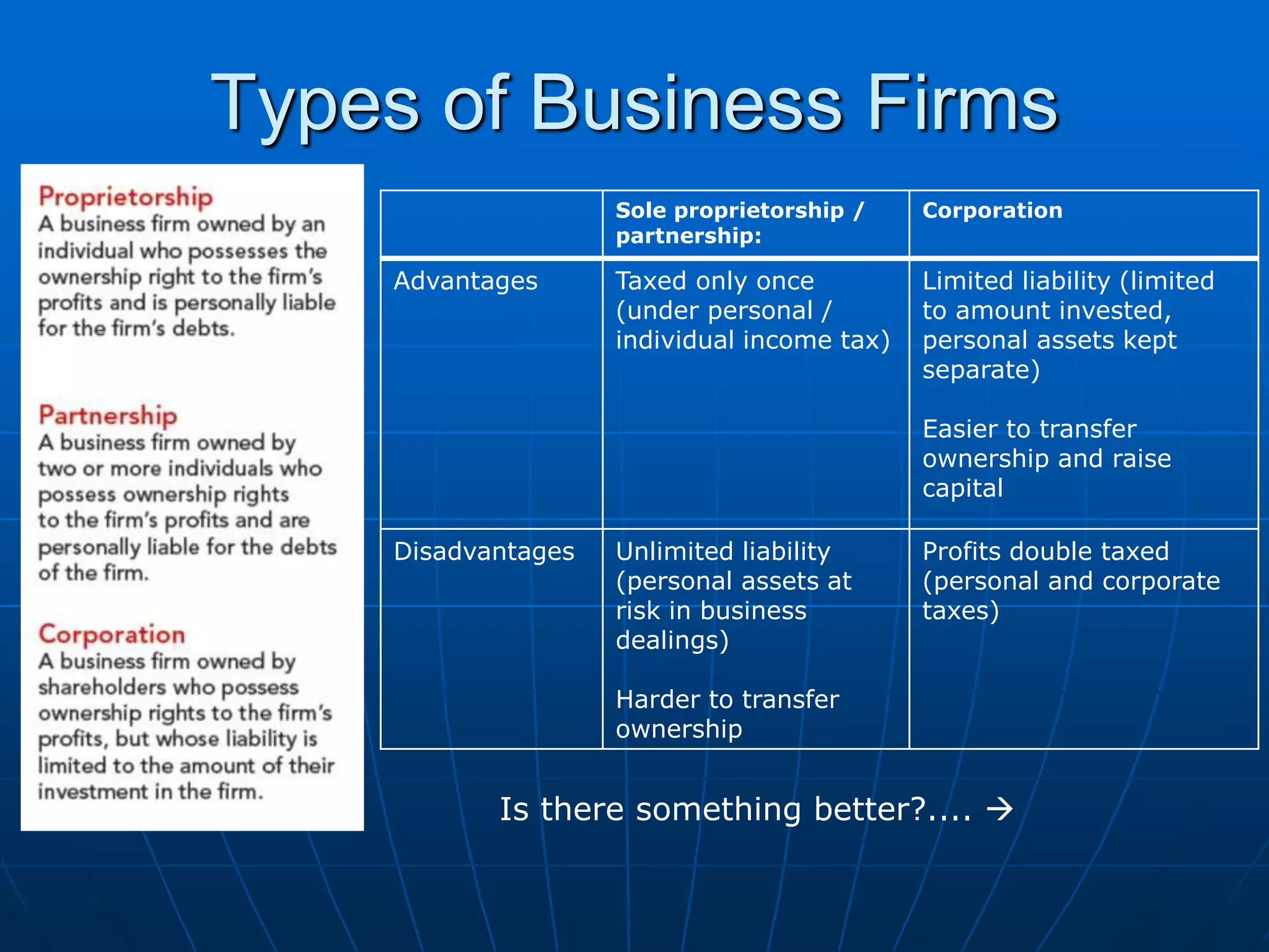
Types of Business Firms
Sole proprietorship /
partnership:
Corporation
Advantages Taxed only once
(under personal /
individual income tax)
Limited liability (limited
to amount invested,
personal assets kept
separate)
Easier to transfer
ownership and raise
capital
Disadvantages Unlimited liability
(personal assets at
risk in business
dealings)
Harder to transfer
ownership
Profits double taxed
(personal and corporate
taxes)
Is there something better?.... 

LLC (Limited Liability Company)
 Since 1977, an increasing number of
states allow a hybrid form of
business organization called the
limited liability company (LLC),
which combines the advantages of
limited liability of a corporation but
the tax advantages of a sole
proprietorship or partnership.

Calculating Economic Costs & Profits
 Economists calculate profit differently than
accountants.
 New terminology: “Economic Costs” vs. “Accounting
Costs” & “Economic Profit” vs. “Accounting Profit”
 The big difference is how you handle opportunity
costs.
 Accountants follow tax laws and associated accounting
standards.
 Economic profits & losses are a much better predictor
of whether a firm will stay in business or not.
Consider this example… 

Test Yourself
If you were the CEO a corporation with
multiple plants….
Would you keep $1 billion invested in a
plant that made an accounting profit of
$500,000 per year? Why or why not?

Another example…
Should I Grow
Soybeans or Corn?
 Suppose you grow soybeans and have an accounting profit
of $40,000 but your neighbors grown corn and have an
accounting profit of $100,000 per year on the same amount
of land.
 If this differential is true industry / nationwide how will the
two industries adjust through time?
 Farmers will leave one industry and enter the other, as they
do prices & profits will adjust until the profit rates are
EQUAL. When this happens there is ZERO ECONOMIC
PROFIT. And this is the ‘long-run equilibrium’.

The Basic Logic You Need to Know
 To remain in business a firm must do at least as well as it
could elsewhere….Otherwise the owners would leave and
pursue those other opportunities.
 “how well it could do elsewhere” is exactly what “opportunity
cost” measures.
 “Economic profit” is based on a measure of “economic costs”
that include these opportunity costs (accountants do not
include them)
 Thus, economic profit measures how well you are doing
MINUS how well you could be doing in your next best
alternative.
 When economic profit is positive you are doing better than
your next best alternative. When it is negative (economic
loss) you could do better elsewhere.

Now… moving on to terminology
 The implicit / opportunity costs
we include in economic costs
(that are not included in
accounting costs due to tax
rules are) are:
• Forgone interest or the forgone
‘normal rate of return’ that could
be earned elsewhere on owner’s
money invested in the business
(‘Opportunity Cost of Equity
Capital’)
• Forgone wages (‘Opportunity
Cost of Owner’s Labor’… the
wages the owners could earn
elsewhere instead of the profit of
the firm they own)

More terminology…
Economic profits are always lower than
Accounting profits because economists
include more costs than accountants
do.
Let’s look at an example with data… 

Test Yourself
Answer  (next slide)

Test Yourself
Accounting Profit = Total Revenue – Accounting Costs
$40,000 = $100,000 - $60,000
Forgone interest (opp. cost of equity capital) = $20,000 x 10% = $2,000
Forgone wages (opportunity cost of owner’s labor) = $28,000
So $30,000 of additional implicit opportunity costs ($28,000+$2,000)
Economic Costs = Accounting Costs + Opportunity Costs = $90,000
Economic Profit = Total Revenue – Economic Costs
$10,000 = $100,000 - $90,000
 So, Mary is doing $10,000 better than her next best alternative

The ‘Short Run’ and ‘Long Run’
 The short run is that period of time during which at least
one input or ‘factor of production’ (usually the size of the
firm’s plant), cannot be changed. The length of the ‘short
run’ varies across industries and firms.
 The long run is a time period long enough for a firm to alter
all of its inputs (or ‘factors of production’), including plant
size and for new firms to enter (or existing firms to exit) the
market.
 Entry & exit are LONG RUN phenomenon. You can close
your doors in the short run, but do not have time to divest
of your assets. We will return to this in the next chapter.

Productivity & Costs in the Short Run
 In the short run a firm’s
productivity, and thus costs
are driven by an economic
law known as “The Law of
Diminishing Returns”
How long can a restaurant keep producing
more by adding more cooks to the kitchen?

Some Productivity Measures
Graphically… 

Graphically…
GPA 
example
Tip: Marginal
always passes
through the
maximum or
minimum of
an average
curve

GPA example..
 What does the “A” in GPA stand for?
AVERAGE
 It is pulled by your MARGINAL
grades up or down.
 Example: Both Erin & Pablo have a
3.0 heading into my class. Erin
makes an A (4.0), Pablo makes a C
(2.0) how does this affect their
Grade Point Averages (GPAs)?

Here are the ones
from the textbook
just to show you
some drawn a bit
better, but they
use a different
example and
numbers.

For those who have had calc…
(not on test/quiz)
 Marginal product is simply the partial
derivative of total product function
with respect to the quantity of labor…
 TP=f(L,K), so MPL=𝜕𝑇𝑃/𝜕𝐿
 Which means it is the slope of the line
tangent to the TP curve… 

Turning to Costs
A firm’s cost are
driven by its
productivity
(inversely)
Marginal cost is
the ‘flip’ of
marginal product
Let’s see…
Productivity
Measures
Cost
Measures
AP
MP
MC
AC
So point of diminishing
returns can be found
here too! Min. of MC

Total Cost can be separated into Total Variable Cost
(TVC) and Total Fixed Cost (TFC)
Because “fixed” factors are fixed in the short run, Total Fixed Cost
does NOT change with output in the short run.

Marginal Cost
This is the one on which decisions on output
levels are made. It’s the one driven by the
law of diminishing returns (marginal
productivity) shown earlier.

Average Costs
 Average costs are the “per unit”
costs. We find each by dividing the
Total by the level of output “Q”

$180÷4=$45 $100÷4=$25 $80÷4=$20
AFC always declines
with output… because
TFC is fixed and you
keep dividing it by a
larger Q.

Graphs
Most of the
time we use
this we do so
graphically,
and without
specific
numbers so
the areas are
important to
learn.

Here are the ones from the textbook just to show you
some drawn a bit better, but they use a different example
and numbers.
For those who know calculus those same ideas apply, MC
is derivative (or tangent line) of TC, and Average costs
are the ray from the origin…

Also, note again, that MC pulls the average curves (both
of them). It passes through their minimums (both).
When MC<AVC (or ATC) it pulls it down, when MC>AVC
(or ATC) it pulls it up.
Both ATC
and AVC
are rising
because
MC is
greater
than both
Both ATC
and AVC
are falling
because
MC is less
than both
ATC falling
and AVC
rising
because
MC>AVC
but
MC<ATC

U-shape of ATC…
 When output is small, per-unit cost (ATC) will be high
because of high fixed costs per unit (AFC is high).
 When output is large, per-unit cost (ATC) will be high
because of high MC (due to diminishing returns).
 Thus, the short-run ATC curve will be U-shaped.
 Where ATC is at a minimum is where the firm is most
efficient [“the per unit cost of production are lowest”].
Firm is most
efficient here (per
unit cost lowest)

Test Yourself
Answers (one at a time , 1(a) only next)

Test Yourself
Answers (one at a time )
TC
140
200
280
380
500
Answer for 1(a)
AFC=TFC/Q=$100/5=$20
AVC=TVC/Q=$400/5=$80
ATC=TC/Q=$500/5=$100…or
ATC=AFC+AVC=$20+$80=$100

Test Yourself
TC
140
200
280
380
500
Answer for 1(b)
TC(3) – TC(2) = $280-$200=$80
Answer for 1(a)
AFC=TFC/Q=$100/5=$20
AVC=TVC/Q=$400/5=$80
ATC=TC/Q=$500/5=$100…or
ATC=AFC+AVC=$20+$80=$100

Test Yourself
Answers (one at a time  1(a) only next)

Test Yourself
Minimum of MC
(corresponds to
maximum of MP)
Occurs at an
output level of 2
units
=2

Test Yourself
Answer for 2(b)
TFC=TC-TVC=$150-$145=$5
=2
=$5

Test Yourself
Answer for 2(b)
TFC=TC-TVC=$150-$145=$5
Answer for 2(c)
AFC=TFC÷Q=$5÷5=$1
=2
=$5
=$1

Test Yourself
Answer for 2(d)
TFC=TC-TVC=$30-$25=$5
Same as it was at an
output level of 5 units
in Question 2(b)!
TFC is the same at all
levels of output.
=2
=$5
=$1
=$5

Test Yourself
=2
=$5
=$1
=$5
ATC
--
20÷1= $20
30÷2= $15
60÷3= $20
100÷4= $25
150÷5= $30
Occurs at an
output level of 2
units
=2

Test Yourself
5
7
3
6
2
?
?
?
AFC=$2

Test Yourself
5
7
3
6
2
?
? ?
?
10
25
35
If
ATC = TC ÷ Q
Then
ATC×Q=TC
Same for
other totals
These are the
areas.
TVC=$25
TFC=$10
Combined Area
is TC=$35

Test Yourself
5
7
3
6
2
?
2.50
1
10
25
35
TFC is the
same at all
levels of
output, then
compute the
AFC’s from it.
? ?
10
10

Test Yourself
5
7
3
6
2
60
? 2.50
1
10
25
35
? ?
7
?
10
10
70

Test Yourself
5
7
3
6
2
60
? 2.50
1
10
25
35
?
7
?
10
10
70
32

Test Yourself
5
7
3
6
2
60
2.50
1
10
25
35
7
10
10
70
32 22 8 5.50

Shifts in the Cost Curves
 Resource prices
 Taxes
 Regulations
 Technology

Output & Costs in the Long Run
 In the long run EVERYTHING is
variable (there are no fixed costs),
and there is time for firms to exit &
enter the industry.
 Let’s look at how costs change when
you change your plant size (the thing
that was fixed before… the number
of garbage trucks in my example)

Economies of Scale
Mass production
Specialization
Learning by
doing
Other cost
sharing
efficiencies

Different Industries Are Different
 This determines firm size & number
of firms in the industry

Sunk Costs
 Erin paid $100 for a share of stock and the price has
fallen to $60. She expresses unwillingness to sell the
stock until it goes back up to at least $100. Should
the original price influence her current decision to
hold or sell the stock?
 What is the right criteria for deciding whether to sell
or hold a stock you own?
Sunk Costs should never be
considered when making
decisions.
They can inform future choices
but are not now relevant.

Test Yourself
 Suppose you paid a $75 non-refundable fee to attend an
upcoming cooking class, but right before it starts a better
opportunity arises—a long-lost friend calls who is only in
town for one night and wants to get together. Should you
tell your friend “no” simply because you already paid for
the class?
 Lastly, consider a road construction project expected to
cost $50 million and create $65 million in benefits. Near
completion, after $50 million is spent, an unexpected cost
results in an additional $25 million needed to complete the
project or the road is unusable. Should it be completed
even though the new total cost of $75 million is greater
than the total benefit?
 In retrospect, the road should not have been built. But one
cannot go back in time. Whether the road is currently
worth finishing is an entirely new and different decision.

Principle of microeconomic.pptx

Principle of microeconomic.pptx

More Related Content

Similar to Principle of microeconomic.pptx

Recently uploaded

Principle of microeconomic.pptx