Implementation of a high-resolution regional ocean modeling system (ROMS) for the study of air-sea interaction of the Bay of Bengal

The goal of this study is to develop a High-resolution Regional Ocean Model and implement it with the help of the Regional Ocean Modeling System (ROMS) for the Bay of Bengal which is a tropical ocean basin with three sides covered by land and an Open Ocean on the south side. A new generation of sophisticated ocean circulation ROMS has been specially customized for accurate simulation of the Bay of Bengal ocean systems. It covered a wide range of features including higher-order advection schemes, accurate and efficient physical and numerical algorithms, and several subgrid-scale parameterizations, atmospheric, oceanic, and benthic boundary layers, several coupled models for atmosphere, ocean, biogeochemical, and ecosystem responses. Besides, ROMS produced a large amount of data depicting various properties of the ocean such as water temperature, flow velocity, water density, and salinity, etc. The model outputs showed that the upper layer circulation of the Bay of Bengal is subjected to strong seasonal variability. During the early northeast monsoon in November, the large-scale flow pattern in the bay is cyclonic and the western boundary current, the East Indian coastal current (EICC) flows southward from the Bengal shelf north of 200N to the east coast of Sri Lanka. A cyclonic gyre that forms in the southwestern Bay of Bengal during October. In December it covered almost the whole bay from 84ºE to 93ºE and 8ºN to 18ºN. It dies off until late April where we can only see a cyclonic eddy centered at 12ºN 86ºE. At the end of June, the circulation in the Bay is mainly anticyclonic and dominated by four eddies centered at 10ºN 83ºE, 11ºN 86ºE, 15ºN 91ºE1, and 8ºN 86ºE. During July these anticyclonic eddies move towards the west of the bay and by the end of August, the anticyclonic circulation of the Bay is confined to the west of the bay. In September the anticyclonic gyre is much smaller and to the north of the Bay. The freshwater plume along the northwest part of the Bay is well reproduced by the model even if the river discharge was not included in the model. It does not advect towards the interior of the bay not until the end of the southwest winds. The represented model also shows the seasonal cycle of the surface temperature. And this modeling tried to resolve some important atmospheric and oceanic features in reasonable ways, analyzed and presented in this research. Some parameters such as temperature and salinity profiles were verified with model and Argo data in the area of the Bay of Bengal.

Recommended
More Related Content
What's hot
What's hot (20)
Similar to Implementation of a high-resolution regional ocean modeling system (ROMS) for the study of air-sea interaction of the Bay of Bengal
Similar to Implementation of a high-resolution regional ocean modeling system (ROMS) for the study of air-sea interaction of the Bay of Bengal (20)
More from Hafez Ahmad
More from Hafez Ahmad (20)
Recently uploaded
Recently uploaded (20)
Implementation of a high-resolution regional ocean modeling system (ROMS) for the study of air-sea interaction of the Bay of Bengal
- 1. Implementation of a high-resolution regional ocean modeling system (ROMS) for the study of air-sea interaction of the Bay of Bengal A Term Paper Submitted for the compilation of the course OCEAN-416 4th year B.Sc. (Hon’s) Examination, 2018 In Oceanography SUBMITTED BY Hafez Ahmad Examination Roll: 15207021 Session: 2014-15 Year of Examination: 2018 Examination held in 2020 Department of Oceanography University of Chittagong Chattogram-4331, Bangladesh 16 February 2021
- 2. i Recommendation This is to certify that term paper entitled “Implementation of a high-resolution regional ocean modeling system (ROMS) for the study of air-sea interaction of the Bay of Bengal” is an original research work, Hafez Ahmad, ID No. 15207021, Department of Oceanography, Faculty of Marine Sciences and Fisheries, University of Chittagong, conducted under my supervision. I also certify that this research work presented here is suitable for submission as to its style and contents for the fulfillment of the requirement for the degree of B.Sc. (Hons) in Oceanography. Supervisor Md. Enamul Hoque Assistant Professor Department of Oceanography Faculty of Marine Sciences and Fisheries University of Chittagong, Bangladesh Chairman Dr. Mohammad Muslem Uddin Department of Oceanography Faculty of Marine Sciences and Fisheries University of Chittagong, Bangladesh
- 3. ii Declaration This dissertation is being submitted in fulfillment of the requirements for the B.Sc. degree of Oceanography for the Term paper (OCEAN 416) at the Department of Oceanography, University of Chittagong, and Chittagong, Bangladesh. The term paper is the result of my own independent work, except otherwise stated. Other sources are acknowledged in the text giving explicit references also a bibliography is appended. I hereby give consent for my dissertation, if accepted, to be made available for photocopying and for interlibrary loan and the title and summary to be available to outside organizations. Signed Hafez Ahmad
- 4. iii Acknowledgments I would like to express my gratitude to the people at the University of Chittagong, Bangladesh for continually providing the necessary means that allowed me to do this research. I would like to thank the people who on different occasions helped me to collect and process scientific data with paramount importance for this work who provided the hydrography data for the Bay of Bengal, who provide field based atmospheric data, who ventured going with me, and who showed me some python tricks at the beginning of my term paper. Many people helped me during my journey in the United States at Florida Gulf Coast University, Florida in too various ways. My special thank belongs to my supervisor, Md. Enamul Hoque (Assistant Professor, University of Chittagong, Bangladesh) for the continued guidance and great recommendations. Great thanks got to my parents for making every effort to provide me with the best education possible. I thank my friends with indefinite love and patience gave me the strength to survive my time in Chittagong. Last but not the least, I thank Allah in all forms for shinning the torch in the tunnel nothing about this would have been possible without Him.
- 5. iv Implementation of a high-resolution regional ocean modeling system (ROMS) for the study of air-sea interaction of the Bay of Bengal Faculty of Marine Sciences and Fisheries Department of Oceanography University of Chittagong Abstracts The goal of this study is to develop a High-resolution Regional Ocean Model and implement it with the help of the Regional Ocean Modeling System (ROMS) for the Bay of Bengal which is a tropical ocean basin with three sides covered by land and an Open Ocean on the south side. A new generation of sophisticated ocean circulation ROMS has been specially customized for accurate simulation of the Bay of Bengal ocean systems. It covered a wide range of features including higher-order advection schemes, accurate and efficient physical and numerical algorithms, and several subgrid-scale parameterizations, atmospheric, oceanic, and benthic boundary layers, several coupled models for atmosphere, ocean, biogeochemical, and ecosystem responses. Besides, ROMS produced a large amount of data depicting various properties of the ocean such as water temperature, flow velocity, water density, and salinity, etc. The model outputs showed that the upper layer circulation of the Bay of Bengal is subjected to strong seasonal variability. During the early northeast monsoon in November, the large-scale flow pattern in the bay is cyclonic and the western boundary current, the East Indian coastal current (EICC) flows southward from the Bengal shelf north of 200 N to the east coast of Sri Lanka. A cyclonic gyre that forms in the southwestern Bay of Bengal during October. In December it covered almost the whole bay from 84ºE to 93ºE and 8ºN to 18ºN. It dies off until late April where we can only see a cyclonic eddy centered at 12ºN 86ºE. At the end of June, the circulation in the Bay is mainly anticyclonic and dominated by four eddies centered at 10ºN 83ºE, 11ºN 86ºE, 15ºN 91ºE1, and 8ºN 86ºE. During July these anticyclonic eddies move towards the west of the bay and by the end of August, the anticyclonic circulation of the Bay is confined to the west of the bay. In September the anticyclonic gyre is much smaller and to the north of the Bay. The freshwater plume along the northwest part of the Bay is well reproduced by the model even if the river discharge was not included in the model. It does not advect towards the interior of the bay not until the end of the southwest winds. The represented model also shows the seasonal cycle of the surface temperature. And this modeling tried to resolve some important atmospheric and oceanic features in reasonable ways, analyzed and presented in this research. Some parameters such as temperature and salinity profiles were verified with model and Argo data in the area of the Bay of Bengal.
- 6. v Table of Contents Chapter One........................................................................................................................1 Introduction ........................................................................................................................1 1.2 Aims and objectives...................................................................................................7 Chapter Two........................................................................................................................8 Literature review.................................................................................................................8 General circulation in the Bay of Bengal..........................................................................9 2.1 Wind Pattern Northern Bay of Bengal.......................................................................9 2.2 Hydrology and Nutrient discharge...........................................................................10 2.3 Waves, Tides, and Currents in the region and their role in nutrients distribution ...12 2.4 Cyclones and their intensification............................................................................13 Chapter Three ...................................................................................................................14 3.1 Study area....................................................................................................................14 3.2 Data, model, and methodology....................................................................................14 3.2.1 River discharge data...........................................................................................14 3.2.2 Currents data......................................................................................................15 3.2.3 Model description and Configuration................................................................15 3.2.4 Grid Generation .................................................................................................16 3.2.5 Initial conditions and external forces.................................................................16 3.2.6 Buoyancy forcing...............................................................................................16 3.2.7 Surface and bottom flux of momentum.............................................................17 3.2.8 Boundary conditions..........................................................................................17 3.2.9 Lateral and vertical mixing................................................................................17 3.2.10 Numerical kernel..............................................................................................17 3.2.11 Sub-models ......................................................................................................17 3.2.12 Adjoint based algorithms and data assimilation..............................................17 3.2.13 Installation and running processes...................................................................19 Chapter Four ....................................................................................................................21 Implementation and analysis of the ROMS’s Simulated results and Discussions ........21 4.1 Wind circulation.......................................................................................................21 4.2 General circulation of the Bay of Bengal.................................................................21
- 7. vi 4.3 Movement of Temperature and salt .........................................................................23 4.4 Comparison of simulations with drifter and Argo data and evaluation...................24 Chapter Five......................................................................................................................26 Conclusion ........................................................................................................................26 Chapter Six........................................................................................................................27 References.........................................................................................................................27 List of Figures Figure 1. Typical S Coordinate system .....................................................................................................4 Figure 2. Hybrid z − σ Coordinate ...........................................................................................................5 Figure 3. Typical Hybrid z-coordinate system toward the S-coordinate system ..................................5 Figure 4. ROMS grid for the Bay of Bengal.............................................................................................6 Figure 5. Schematic map of the Northeast monsoon and southwest monsoon......................................9 Figure 6. Freshwater discharges (m3 s−1) from the seven major rivers in the BoB ...........................10 Figure 7. The annual cycle of rainfall, evaporation, and river discharge from all major rivers flowing into the BoB .................................................................................................................................11 Figure 8. Bathymetric Map of the Bay of Bengal...................................................................................14 Figure 9. The main component of the Regional Ocean Modeling System ...........................................15 Figure 10. Schematic Work Floe of the Regional Ocean Modeling System.........................................16 Figure 11. Set up and files of the Regional Modeling System in the local computer ..........................18 Figure 12. Circulation in the entire BoB in three different seasons ....................................................22 Figure 13. Movement of surface current in three different seasons.....................................................23 Figure 14.Vertical transects of Salinity...................................................................................................24 Figure 15. The figure of the comparison of the ROMS and Argo data of the temperature...............25 List of Tables Table 1. The boundary conditions.............................................................................................................2 Table 2. Some existing oceanographic models in different countries.....................................................6 Table 3. The programming framework of ROMS ( initialize, run, and finalize)................................18 Table 4. Numerical parameters used in ROMS model simulation.......................................................19
- 8. 1 Chapter One Introduction The ocean covers more than 70% of the earth’s surface and has fascinated humans in many ways since the ancient period. Modern oceanography studies cover many aspects of the ocean. However, the observation of the oceanographic phenomena is very crucial that is generally made from satellites that are restricted to the surface and those made by boast and drifter are sparse due to the vastness of the ocean. With the help of the digital computer, an array of numerical ocean models has been developed to facilitate research in one or several subfields of oceanography. These models overcome the existing problems when it comes to the solution of the equations of motion. Simulation models can calculate realistic oceanic circulation either horizontal or vertical direction by resolving the primitive equations coupled with the international equation of the state of the sea, as well as the equations temperature and salt conservation (Maria, 2012). Furthermore, the importance of predicting the state of the ocean currents, tide, temperature, salinity, and sea level in real time has been recognized years ago in many modern developed countries for their different regional and global purposes. Different ocean models can be loosely characterized by their approaches to spatial discretization and vertical coordinate treatment. Among them, the Regional Ocean modeling system (ROMS) is a free surface, hydrostatic primitive equations, and terrain- following ocean model. It was based on the S-coordinate Rutgers university model by Song haidvogel (1994). ROMS can be coupled to wave and atmosphere models for a more complete prediction of the hydrostatics parameters (Costa et al., 2020). We assume that seawater is an incompressible fluid which is equivalent to the Boussinesq approximation that also assumes density is relatively constant in space and time except when it is multiplied by the gravity acceleration in calculations of pressure. It is written in FORTRAN 90/95. It uses C- preprocessing to activate the various physical and numerical options. The basic Equations frequently used as fundamental mathematical calculations in Oceanography are given below. 1. Hydrostatic equation − 𝜕𝑃 𝜕𝑡 − 𝜌𝑔 = 0 − − − − − − − −(1) 𝑤ℎ𝑒𝑟𝑒, 𝑃: 𝑃𝑟𝑒𝑠𝑠𝑢𝑟𝑒, 𝑔: 𝑔𝑟𝑎𝑣𝑖𝑡𝑎𝑡𝑖𝑜𝑛𝑎𝑙 𝑎𝑐𝑐𝑒𝑙𝑒𝑟𝑎𝑡𝑖𝑜𝑛 2. Continuity equation 𝜕𝜌 𝜕𝑡 + 𝜕𝜌𝑢 𝜕𝑥 + 𝜕𝜌𝑣 𝜕𝑦 + 𝜕𝜌𝑤 𝜕𝑧 = 0 − − − − − − − −(2) 𝑤ℎ𝑒𝑟𝑒, Velocity components: (u, v, w), ρ: density, coordinates: (x, y, z) 3. Conservation of temperature 𝜕𝑇 𝜕𝑡 + 𝑈. ∇𝑇 = 𝐾ℎ∇ℎ 2 𝑇 + 𝐾𝑣 𝜕2 𝑇 𝜕𝑧2 − − − − − − − −(3)
- 9. 2 4. Conservation of salt 𝜕𝑆 𝜕𝑡 + 𝑈. ∇𝑆 = 𝐾ℎ∇ℎ 2 𝑆 + 𝐾𝑣 𝜕2 𝑆 𝜕𝑧2 − − − − − − − −(4) 𝑤ℎ𝑒𝑟𝑒; 𝐾ℎ: 𝑐𝑜𝑒𝑓𝑓𝑖𝑐𝑖𝑒𝑛𝑡 𝑜𝑓 𝑣𝑖𝑠𝑐𝑜𝑠𝑖𝑡𝑦, 𝑈: 𝑣𝑒𝑙𝑜𝑐𝑖𝑡𝑦 5. State equation 𝜌 = (𝑇, 𝑆, 𝑝) − − − − − − − −(5) 𝑤ℎ𝑒𝑟𝑒; 𝑇: 𝑇𝑒𝑚𝑝𝑒𝑟𝑎𝑡𝑢𝑟𝑒, 𝑆: 𝑆𝑎𝑙𝑖𝑛𝑖𝑡𝑦, 𝑝: 𝑝𝑟𝑒𝑠𝑠𝑢𝑟𝑒 ROMS solves the Reynolds averaged Navier-Stokes equation using the hydrostatic and Boussinesq assumptions (Thyng et al., 2020). If the ocean initial state (velocity, temperature, etc.) is known at a specific given time along with the boundary conditions of the surface, bottom, and lateral sides then the ocean state at a subsequent time can be determined. 6. Navier-Stokes equations of fluid dynamics in the three-dimensional, unsteady form(Nancy Hall, 2015). 𝑋 − 𝑀𝑜𝑚𝑒𝑛𝑡𝑢𝑚; 𝜕𝜌𝑢 𝜕𝑡 + 𝜕𝜌𝑢2 𝜕𝑥 + 𝜕𝜌𝑢𝑣 𝜕𝑦 + 𝜕𝜌𝑣𝑤 𝜕𝑧 = − 𝜕𝑝 𝜕𝑥 + 1 𝑅𝑒𝑟 [ 𝜕𝜏𝑥𝑥 𝜕𝑥 + 𝜕𝜏𝑥𝑦 𝜕𝑦 + 𝜕𝜏𝑥𝑧 𝜕𝑧 ] … . (6) 𝑌 − 𝑀𝑜𝑚𝑒𝑛𝑡𝑢𝑚; 𝜕𝜌𝑣 𝜕𝑡 + 𝜕𝜌𝑣𝑢 𝜕𝑥 + 𝜕𝜌𝑣2 𝜕𝑦 + 𝜕𝜌𝑣𝑤 𝜕𝑧 = − 𝜕𝑝 𝜕𝑦 + 1 𝑅𝑒𝑟 [ 𝜕𝜏𝑥𝑦 𝜕𝑥 + 𝜕𝜏𝑦𝑦 𝜕𝑦 + 𝜕𝜏𝑦𝑧 𝜕𝑧 ] … . (7) 𝑍 − 𝑀𝑜𝑚𝑒𝑛𝑡𝑢𝑚; 𝜕𝜌𝑤 𝜕𝑡 + 𝜕𝜌𝑢𝑤 𝜕𝑥 + 𝜕𝜌𝑣𝑤 𝜕𝑦 + 𝜕𝜌𝑤2 𝜕𝑧 = − 𝜕𝑝 𝜕𝑦 + 1 𝑅𝑒𝑟 [ 𝜕𝜏𝑥𝑦 𝜕𝑥 + 𝜕𝜏𝑦𝑦 𝜕𝑦 + 𝜕𝜏𝑦𝑧 𝜕𝑧 ] … . (8) Here, coordinates: (x, y, z) ; time =t; pressure: P; heat flux= q Velocity components: (u, v, w): density= ρ ; stress: τ; Reynolds number: Re Table 1. The boundary conditions Surface boundary conditions (z=n) Bottom boundary conditions (z=-H) 7: Kinematic 𝜕𝜂 𝜕𝑡 = 𝑤 11: Kinematic 𝑤 = −𝑢. ∇𝐻 8: Wind stress 𝐴𝑣 𝜕𝑢 𝜕𝑧 = 𝜏𝑠𝑥 𝐴𝑣 𝜕𝑣 𝜕𝑧 = 𝜏𝑠𝑦 12: Bottom friction 𝐴𝑣 𝜕𝑢 𝜕𝑧 = 𝜏𝑏𝑥 𝐴𝑣 𝜕𝑣 𝜕𝑧 = 𝜏𝑏𝑥 9: Heat flux 𝐾𝑣 𝜕𝑇 𝜕𝑧 = 𝑄 𝜌0𝐶𝑃 13: Bottom heat flux 𝐾𝑣 𝜕𝑇 𝜕𝑧 = 0 10: Slat flux 𝐾𝑣 𝜕𝑆 𝜕𝑧 = 𝑆(𝐸−𝑃) 𝜌0 14: Bottom salt flux 𝐾𝑣 𝜕𝑆 𝜕𝑧 = 0
- 10. 3 Where Prognostic variables of these equations are u, v, S, T, η (the vertical displacement of the free surface) the diagnostic variables are w, P, ρ and the parameters are Av, Kv. ROMS was completely rewritten to improve both its numeric and efficiency in single and multi- threaded computer architectures. ROMS applied the Boussinesq approximation, meaning that density differences only affect vertical accelerations through the buoyancy term. It uses a split- explicit and stretched terrain-following sigma coordinates in vertical and horizontal Arakawa-C grid which allows for higher resolution at depths of particular interest such as mixed layer. Barotropic momentum equations are solved by implying shorter time steps. The third-order upstream biased advection scheme is implemented in ROMS which helps to generate a steep gradient which further enhances the effective solution for a given grid size (Penven, Marchesiello, Debreu, & Lefèvre, 2008; Shchepetkin & McWilliams, 2005). The air-sea interaction module of the ROMS is based on the bulk formulation and is adapted from the coupled ocean-atmosphere response experiment algorithm for air-sea computation. The bulk formulation is used for standalone or coupled mode with atmosphere models (Fairall, Bradley, Rogers, Edson, & Young, 1996). Coastal boundaries can also be specified as a finite-discretized grid via land/sea masking in the ROMS modeling. As in the vertical, the horizontal stencil utilizes centered, second-order finite differences. However, the code is designed to make the implementation of higher-order stencils easily. It has various options for advection schemes such as second and fourth-order centered differences, and third-order, upstream biased. The later scheme is the model default and it has a velocity-dependent hyper-diffusion dissipation as the dominant truncation error (Shchepetkin and McWilliams, 1998). These schemes are stable for the predictor-corrector methodology of the model. In addition, there is an option for conservative parabolic spline representation of vertical advection which has dispersion properties similar to an eight-order accurate conventional scheme. There are several subgrid-scale parameterizations in ROMS. The horizontal mixing of momentum and tracers can be along with vertical levels, geopotential (constant depth) surfaces, or isopycnic (constant density) surfaces. The mixing operator can be harmonic (3-point stencil) or biharmonic (5-point stencil). Haidvogel and Beckmann (1999) for an overview of all these operators. The vertical mixing parameterization in ROMS can be either by local or nonlocal closure schemes. The local closure schemes are based on the level 2.5 turbulent kinetic energy equations by Mellor and Yamada (1982) and the Generic Length Scale (GLS) parameterization (Umlauf and Burchard, 2003). The nonlocal closure scheme is based on the K-profile, boundary layer formulation by Large et al. (1994). The K-profile scheme has been expanded to include both surface and bottom oceanic boundary layers. The GLS is a two-equation turbulence model that allows a wide range of vertical mixing closures, including the popular k-kl (Mellor-Yamada level 2.5), k-e, and k-w schemes. Several stability functions (Canuto et al., 2001) have been also added to provide further flexibility. Another study (Warner et al., 2005a) evaluated the performance of these turbulence closures in ROMS in terms of idealized sediment transport applications. Besides, there is a wave/current bed boundary layer scheme that provides the bottom stress (Styles and Glenn, 2000) and sediment transport which become important in coastal applications. The main features are high order advection schemes, accurate pressure gradient algorithms, atmospheric, ocean, and benthic boundary layers, several subgrid-scale parameterization biological modules and data assimilation, etc. It has a wide range of applications for example
- 11. 4 integrated ocean modeling uses ROMS for the circulation part and adds other variables and processes of interest. It has extensive pre and post-processing software for data preparation, analysis, and visualization. The whole input and output data structure of the model is via NetCDF which is easy to interchange the data between the computer, user community, and other independent analysis software and visualize. There are two systems of the grid system. They are horizontal grid systems and vertical grid systems. ROMS has a generalized vertical, terrain-following coordinate system. Currently, two vertical transformation equations are available which can support numerous vertical stretching 1D –function, when some constraints, are satisfied. Three main verticals coordinate systems are generally used in most ocean modeling systems. a. Z- coordinates: The vertical coordinate is the depth that can provide the very fine resolution needed to represent three-dimensional turbulent processes. b. Sigma coordinate: This type of coordinate is the most appropriate for the continental shelf and coastal regions where the bottom and the surface boundary layers may merge. c. Isopycnal coordinates: This system divides the water column into distinct homogeneous layers whose thickness can vary from place to place and from one-time step to the next. On the other hand, the Horizontal grid includes finite difference, finite element, and spectral. ROMS can be executed on a stretched orthogonal curvilinear grid with an average resolution of 10 km (Haidvogel et al., 2000). (a) S coordinate system Figure 1. Typical S Coordinate system
- 12. 5 Figure 2. Hybrid z − σ Coordinate (z =absolute depth, σ =normalized depth) Figure 3. Typical Hybrid z-coordinate system toward the S-coordinate system
- 13. 6 Figure 4. ROMS grid for the Bay of Bengal Table 2. Some existing oceanographic models in different countries Acrony m System names Countr y Domains References FKeySH COM Florida Straits, south Florida, and keys hybrid coordinate ocean model USA Florida straits and the south Florida coastal and shelf areas Griffies & Treguier, 2013 NWPS The near shore wave prediction system USA Coastal waters of all US territories Haidvogel & Beckmann, 1999 REMO Oceanographic modeling and observation network Brazil Western equatorial and south Atlantic ocean Kourafalou et al., 2015 WCNRT West coast near real time data assimilation system USA West US coast, California Current system Wilkin et al., 2s005 eReefs eReef Marine modelling Australi a Australian coastal margins Steven et.al, 2019 COSYN A Coastal observation system for northern and arctic seas German y North sea, German bight, German Wadden sea Riethmüller et al., 2009 POSEID ON Regional monitoring and forecasting system Greece Aegean and Mediterranean seas Ray, R. D. (1999). POM Princeton Ocean Model USA Global ocean Ezer,& Mellor, 1997 ROMS The regional ocean modeling system Region al Defined area Song haidvogel (1994).
- 14. 7 1.2 Aims and objectives The main objective of this term paper is to study the community-built regional Model that must be coupled or integrated to the other ocean models and the real-time observing systems to obtain improvement in the representation of ocean circulation in a high or medium-resolution ocean model. The second aim is to determine whether assimilation and planned observational networks can improve circulation estimates of the coastal ocean. From a long-term perspective, I hope to develop a methodology for improving the operational ocean model and for giving recommendations on the design of future oceanographic forecasts of the Bay of Bengal. Specifically, The topmost important objectives of this research work are given below 1. To Make and test a regional ocean modeling framework for relocatable coastal ocean prediction applications on the Bay of Bengal region. 2. To develop advanced 4-dimension Variational (4D-Var) data assimilation capabilities and analysis algorithms for observation sensitivity, observation impact, adaptive sampling, and forecast errors and uncertainties. 3. To show how to Bay of Bengal responds to the physical change of the environment. 4. To recommend types of models appropriate for coastal-specific situations. 5. To develop adjoint-based forecast weather of ocean analysis tools similar to those available in Numerical Weather Prediction for the atmosphere for circulation stability, sensitivity analysis, and ensemble prediction. 6. To build multiple grid nesting capabilities to resolve unique geographical regions and monsoonal as well as localized circulation regimes.
- 15. 8 Chapter Two Literature review Ocean models are numerical models focused on the properties of the ocean and its circulation. Ocean models play a very important role in the understanding of the ocean’s influence on weather and climate. Every ocean model is very an approximation of the absolute physics of the Oceanic features. In some cases, simplifications of the mathematical representations are introduced in order to isolate a subset of the physics believes to essential to the phenomena under study but in all cases computational feasibility demands approximation. Numerical modeling is largely concerned with how to choose approximations and how to analyze their consequences. In choosing one must consider both those approximations that alter the physical system and the approximations involved in converting the continuous equations that describe that system into a discrete set of equations that can be integrated numerically. Models are used for two purposes understanding and simulation or prediction. If the ocean is using a model to understand the ocean it is comforting to know that it is capable of realistic simulations. Yet it is difficult to achieve realistic simulations especially of new conditions without understanding what physics is essential and how to model it (Cane, 1986). Realistic ocean circulation models are usually based on Boussinesq hydrostatic momentum, mass balances, materials tracer conservation, seawater’s equation of state, and parameterized subgrid- scale transports. The motivation to build a free-surface oceanic model is twofold. From a physical point of view, it is desirable to recapture processes lost or altered by the rigid-lid assumption. These include tidal motions, altered dispersion relations for the Rossby waves, etc. (Shchepetkin & McWilliams, 2005). The other motivation comes from computational economics: as pointed out by (Killworth et al., 1991), there is a natural physical ratio of phase speeds for the external and internal gravity-wave modes. Primitive equation-based models are the General circulation model, Ocean circulation which has comprehensive processes parameterizations (Zhang et al., 2020). The oceanic current transport has a profound impact on marine life, ocean biogeochemical processes, basin ecosystem, fishery, and other relevant industries. Ocean current is a significant parameter that helps to move not only marine organisms around the ocean but also distributes heat and nutrients. Thus the determination of the current pathway, localized impacts, and effects of distance weather is essential, it is only possible with the Ocean model with the large simulation of exact ocean weather conditions (Sen et al., 2020). So, a good understanding of the wind pattern, circulation, localized currents of the ocean, and coastal waters is a prerequisite for designing and developing Ocean models and forecasting systems. Regional Ocean Modeling System is one of the models that can serve purposes because it is a three-dimensional, terrain-following sigma-coordinate ocean model that solves the primitive equations based on Boussinesq and hydrostatic balance approximations (Day et al. 2020).
- 16. 9 General circulation in the Bay of Bengal 2.1 Wind Pattern Northern Bay of Bengal Circulation dynamics and marine productivity in the northern Bay of Bengal (BoB) are controlled by the seasonally reversing wind system called the monsoon. The pre-monsoon season occurs from March to May and is followed by summer monsoon dominating the Indian sub-continent during June-September. Post-monsoon (October to November), north-east monsoon (October to December) (Prakash & Pant, 2019), commonly known as winter monsoon blows from land to sea, whereas south-west monsoon (June to September) (Vinayachandran & Kurian, 2007), known as summer monsoon blows from sea to land, which brings a steady stream of moisture that triggers the torrential rainy season in the region. SW monsoon contributes 80% of the annual rainfall over the Indian subcontinent (Saikranthi, Radhakrishna, Thota, & Satheesh, 2019). The circulation in the BoB is also affected by remote equatorial Indian Ocean, monsoon, and freshwater inputs. a well-developed anticyclone gyre and poleward east India coastal current can be found in the BoB during pre-monsoon (February to May) (Shetye et al., 1993). In regular summer monsoon, the westerly winds along the equator push warmer water along the coast via equatorial downwelling and coastally trapped Kelvin waves. This process opposes the cooling tendencies by evaporation, coastal upwelling and oceanic heat advection which are brought by the alongshore winds off the coast (Saji, Goswami, Vinayachandran, & Yamagata, 1999). Indian Ocean Dipole (IOD) is strongly dependent on the strength of monsoon circulation and its variability affects greatly this mode. Negative IOD brings warmer water by shifting trade winds and increasing convergence in the west and greater precipitation in the eastern Indian Ocean and cooler and drier in the west whereas positive brings opposite conditions (warmer and rainy conditions). Warmer SST intensifies the precipitation and wind anomaly to the east. Webster et al. found that the correlation between mean equatorial SST and El Niño-Southern Oscillation (ENSO) is +0.52 in the Indian ocean (Webster, Moore, Loschnigg, & Leben, 1999). Figure 5. Schematic map of the Northeast monsoon and southwest monsoon
- 17. 10 2.2 Hydrology and Nutrient discharge Freshwater influx together with monsoon winds has a strong influence on the circulation dynamics and stratification in the northern BOB. During the SW monsoon, the river influx getting doubled in the bay nearly 183*1011 m3 (Howden & Murtugudde, 2001). The rivers of Bangladesh alone supplies 1,222 million cubic freshwaters into the northern part of the Bay. Northern bay experiences the highest river discharge during SW monsoon when the SW monsoon rainfall is normally at the peak and it's minimum during the winter and pre-monsoon (Seo, Xie, Murtugudde, Jochum, & Miller, 2009). The western and northern regions of the bay experience near-surface temperature inversion in the boreal winter due to the rapid cooling of the surface layer (Thadathil et al., 2002). Figure 6, includes monthly discharge rates of seven rivers (Brahmaputra, Ganga, Irrawaddy, Godavari, Mahanadi, Krishna, and Cauvery) which are the main major sources of nutrients of the BoB. From the figure, monthly river discharge has a maximum between July- September months when it receives strong and organized winds from southwesterly direction and high precipitation (Figure 7). The river's discharge begins decreasing after the monsoon and reaches its minimum during the winter and premonsoon season (March –April). Figure 6. Freshwater discharges (m3 s−1) from the seven major rivers in the BoB (Dey et al., 2020). The discharge of GBM is the combined discharge of Ganges, Brahmaputra, and Meghna.
- 18. 11 Figure 7. The annual cycle of rainfall, evaporation, and river discharge from all major rivers flowing into the BoB (Amol et al., 2019). Open ocean salinity oscillates from 32ppt to 34.5ppt and in the northern coastal region, salinity varies from 10ppt to 25ppt. but at the river mount salinity decreases to 5ppt or even less. During summer salinity decreases up to 1ppt and increases up to 15ppt to 20ppt in winter(Rahman, 2007). During the SW monsoon, this bay receives more than 90% of the freshwater discharge due to heavy rainfall. This enhances riverine nutrients supply and stimulates the phytoplankton concentration in the coastal area of the BoB. High win during SW monsoon strengthens the mixing in the surface waters (Ota et al., 2019). Rivers of the Indian subcontinent provide about 1.74 Teragram (Tg) yr−1 of nitrate, 0.27 Tg yr−1 of phosphate, and 3.58 Tg yr−1 of silicate into the BoB and about 94%, 75%, and 93% of the total nitrogen, phosphate, and silicate fluxes of the total uptake of northern Indian Ocean (Krishna et al., 2016). However, BoB is less productive than the Arabian sea because monsoon winds cannot break the strong stratification which is a consequence of the large freshwater inputs from both river and rainfall (Shenoi, Shankar, & Shetye, 2002). Another factor contributes to becoming a less productive bay in which light penetration is limited due to intense cloud and turbid coastal waters that inhibit photosynthesis in the northern BoB (Bharathi, Sarma, Ramaneswari, & Venkataramana, 2018). Apart from this cyclone eddies and irregular rainfall further influence Chla distribution by breaking stratification. Near the coast, local alongshore current can make coastal upwelling which increases productivity (Thushara & Vinayachandran, 2016). The Ganges Brahmaputra Meghna, Irrawaddy, Godavari, Mahanadi, and Krishna, sittang, and Salween Rivers are the supplier of the main inputs into the Bay. However, 64% of river runoff comes from Ganges Brahmaputra and Meghna river systems. Freshwater and nutrients from the rivers affect greatly the productivity of the bay (Janes, 2018). The Ganges Brahmaputra alone supplies freshwater discharge about ~30742 m3 s-1 and ~ 1*109 tons of sediment per year and the Mahanadi river contributes freshwater discharge of about ~ 2113 m3s-1 and ~60 *106 tons of sediment per year (Milliman et al., 2011). Those rivers, mixing due to
- 19. 12 cyclone and other atmospheric phenomenon such as post-monsoon are the major nutrients such as nitrate, phosphate, and silica supplier to the BoB ( Madhupratapel al., 2002). 2.3 Waves, Tides, and Currents in the region and their role in nutrients distribution Tides have a great influence over marine nutrients cycling in various ways by enhancing the vertical mixing of biomass, suspended matter, nutrients, and making sediment resuspension(Zhao, Daewel, & Schrum, 2019). The topography of BoB is very unique and it has a network of interconnected channels and is exposed to large ocean tides with typical amplitudes of about 2-3 m(Mole, 2012). It has less shelf area on the western boundary and large in the northern and eastern. Therefore tide along the coastline of the BoB is both semi-diurnal and diurnal (Pramanik et al., 2019). The head bay has high surges. The head bay and west coast of BoB experience semi-diurnal tide. The amplitudes of the semi-diurnal tides were reported to double in the head bay (Antony & Unnikrishnan, 2013). At the location of Sundarbans Pussur River and Tiger Point are relatively low due to narrow shelf (Sindhu & Unnikrishnan, 2013). The tide is one of the principal sources of energy that helps in river-driven sediment distribution in the coastal environment. Because it causes changes in the vertical stability of the water column. consequently, in the semidiurnal tidal area, marine organisms like phytoplankton experience two cyclic vertical water mixing(Demers et al., 1986). spatial and temporal sediment distribution of tide-dominated coastal is complex and influenced by river discharge, tidal exchange, and other marine processes (wave, local current, and storm) (Goodbred & Saito, 2012). Tide-dominated Sundarbans cover about half of the northern lower BoB. This was formed by the sediments delivered to the BoB by three rivers (Ganga, Brahmaputra, and Meghna). About 95% of the sediments (100*106 t yr-1) were supplied into the BoB during the SW monsoon from May to September. the tidal range of the Sundarbans area is about 2-4m (Coleman, 1969; Rogers & Goodbred, 2014). A study calculated that ~300 million tons of fluvial sediments are stored on the floodplain, ~750 million tons is discharged at the river mouth and 350 million tons of sediments were thought to go to the deep sea via the Bengal canyon(Rogers, Goodbred, & Mondal, 2013). Coastal sediment movement generally follows along the east coast of India follow monsoon circulation. The coastal circulation is northward during SW monsoon and net sediment transport is from south to north whereas sediment drifts southward with anticlockwise movement during NE monsoon. Though river discharge is low in the non-monsoon period, winds favor upwelling, which causes vertical density gradient and changes internal tide effect-causing suspension of sediment oscillating back and forth by spring and neap tidal cycles. Most of the sediments are transported as suspended load in the fluvial environment and littoral sediment transport and boundary currents spread suspended sediment load are present along the coast and can be thrown off the coast up to 250 km into the deep shelf (Sridhar, Ramana, Ali, & Veeranarayana, 2008). The availability of the in situ wave data over the BoB is very sparse and inhomogeneous. The annual wave height (WH) and speed mostly depend on the seasonal nature of wind reversal. The wave height of the BoB ranges from 0.5 m to 2.5 m. Monthly WH is around 1.8m. WHs in the head Bay are less than 1 m. The upper northern BoB experiences swell and wind waves in the coastal waters with less than 1.5 m WHs during premonsoon due to lower wind speed (4 to 6ms-1 ). Surface winds (2 to 4ms-1 ) are weaker over the BoB during the march. The central or open part of BoB experiences WHs between 1.0m to 1.5 m. October ranges 4 to 6ms-1 WH reduces up to 1.3m. November ~1.2m with 4to 6ms-1 during December, WH over the large areas of the BoB is less than 1.m and the corresponding wind speed range 4 to 6ms-1. During May, the BoB
- 20. 13 experiences enhanced winds and produce higher wave and higher WHs (1.5 to 2m). The winds speed over the central BoB during June ranges between 8 to 10ms-1 and head bay with 6m to 8ms- 1 . July is the roughest month from the annual cycle. On this period, strong wind blow and generates wave (0.5 to 3.5 m). September is the retrieval phase of SW monsoon and wind speed tends to decrease with values between 4 to 6ms-1 (Patra & Bhaskaran, 2016). 2.4 Cyclones and their intensification The BoB is an active zone of Tropical cyclone (TC). Every year, three to four TC occurs which is about 5% of the global TCs (Alam, Hossain, & Shafee, 2003). From 1974 to 2015, about 132 TCs happened in the BoB. The maximum number of TCs occurred during November followed by October, May then December (Bhardwaj, Singh, Pattanaik, & Klotzbach, 2019). There is a link between anthropogenic warming and the weakening of tropical summertime circulation. Kossin analyzed data from 1949to 2016 and provided evidence that TC has slow downed by 10% on average and migrated poleward in several regions especially in the western north pacific. A slowdown of TCs translation speed will enhance local rainfall amounts by the same percentage at all distances from the TC centers (Kossin, 2018). Southwest summer monsoon from June to September brings a major rainy season over the major parts of the Indian subcontinent. With the retreat of the SW monsoon and reversal of the pressure and wind distribution, a low-pressure zone forms over the south BoB. therefore, cyclones form over the low-pressure zone (Kripalani & Kumar, 2004). the zone near the surface and that convert unproductive zone to slightly productive zone (Vinayachandran, 2010). The BoB is usually exposed to tropical cyclones from October to December. Atmospheric convection-driven huge cloud coverage prevailed during cyclones thus make it difficult for the satellite censors to capture ocean color images. Pieces of evidence showed that cyclones intensify and enhance the Chla bloom on the Indian coast. in contrast, the Chla concentration is found low during the years without cyclones (Vinayachandran & Mathew, 2003). After the 1999 cyclone, a sudden increase in the Chla concentration in the northern part of the BoB (Nayak et al., 2001) and cyclone of 2000 caused an increase in Chla in the BoB (K. Rao et al., 2006). Cyclonic eddies are associated with injecting nutrients into the euphotic zone thereby enhance the productivity of the BoB by pushing nutrients into surface waters during southwest monsoon ( Kumar et al., 2004). Most frequent TC occurs during post-monsoon (October to November) due to the presence of weak tropospheric wind shear and stably stratified layer in the upper ocean. Increasing SST leads to an increase in the water vapor content in the atmosphere that is an essential driving force for the cyclone. Cyclonic eddies can increase the primary productivity of BoB through upwelling. Wind-induced processes dominate productivity over the Open Ocean (Southern part). SST is an important parameter that drives the circulation of Ocean current, precipitation, primary productivity, and upwelling, etc. It is affected by several factors such as solar radiation, air-sea interactions, and Ocean currents (Dinesh Kumar, Paul, Muraleedharan, Murty, & Preenu, 2016). It is affected by many oceanic and atmospheric parameters including net incoming solar radiation, air-sea heat exchange, wind stress curl, mixed layer, ocean currents, and advection of eddies(Kumar et al., 2016; Rao et al., 1994; Wilson et al., 2009). Sarangi et al. found that a higher SST range of 290 C to 310 C during October and decreased from November to December because of the impact of freshwater inputs and with northeast monsoonal effect (Sarangi, 2016).
- 21. 14 Chapter Three 3.1 Study area The study covers the entire BoB region between 5.7340 N to 24.3770 N latitude and 78.8980 E to 95.0480 E longitudes. The BoB lies in the far northeast of the Indian Ocean that is surrounded by land (to the north it is bordered by Bangladesh, to the east by Myanmar, and to the west by India and the island of Sri Lanka) except on the south where it is open to the influence of the Indian Ocean. The geographic location of the BoB is between 0o N and 23o N and 80o E and 100o E and covers about 4.087×10⁶ km2 (Madhu et al., 2006). The topography of the BoB is much districted in nature and it has less shelf area on the western side and a very large shelf in the northern region. The bay experiences the major semi-diurnal and diurnal tide (Pramanik et al., 2019). Figure 8. Bathymetric Map of the Bay of Bengal 3.2 Data, model, and methodology 3.2.1 River discharge data The Global Data Runoff Center (GRDC) Data Download portal has been completed and in-situ river discharge data collected since 1988 are available in the Global Runoff Database. They are accessible through the web portal. (https://portal.grdc.bafg.de/applications/public.html?publicuser=PublicUser).
- 22. 15 3.2.2 Currents data The model topography field’s area was extracted from earth topography (etopo2) with 2 min resolution datasets. Finer horizontal resolution 1/90 with 45 vertical levels is considered to simulate the vertical structures of the oceanic parameters accurately. The model is forced with the climatologically varying monthly air-sea fluxes from comprehensive ocean-atmosphere data set (COADS05). Ten major components of tides are forced from TOPEX/POSEIDON global tidal model (TPXO7) to simulate the tidally driven currents as well as sea level. The initial and boundary conditions are taken from the latest 0.250 world ocean atlas 2013 (WOA13). The open oceanic boundary conditions and lateral vertical mixing. The model is simulated for one year to spin up and the results are discussed. 3.2.3 Model description and Configuration The regional ocean model system (ROMS) is an open-source, three-dimensional, free surface terrain-following model widely used by oceanographers to study ocean dynamics over a wide range of spatial (coastal to basin) and temporal (days to seasons, years to decades) scales. The ROMS was chosen as the numerical model in our study area. It is unique because the frameworks include the adjoint-base analysis and prediction tools that are available in numerical weather prediction like 4-dimensional variational data assimilation (4D-Var), ensemble prediction, observations sensitivity and impact, adaptive sampling, and circulation stability and sensitivity analysis. It is freely distributed (http://www.myroms.org) to the earth’s modeling scientific community and has thousands of users worldwide. It follows the Earth System modeling framework (ESMF) conventions for model coupling that is initialized, run, and finalize (Hill, DeLuca, Suarez, Da Silva, & others, 2004). Figure 9. The main component of the Regional Ocean Modeling System
- 23. 16 The ROMS comes with a very modern and modular code written in FORTRAN (F90/95) and uses C-preprocessing to enable the physical and numerical schemes. The model code can be run either serial or parallel with the MPI version which is incorporated in the core. It solves the momentum and transport equations discretized in a three-dimensional frame. The primitive equations were evaluated using boundary-fitted orthogonal, curvilinear coordinates on a staggered Arakawa c grid (Chakraborty & Gangopadhyay, 2015; Pramanik et al., 2019). The ROMS is configured for the BoB region with 256 grid points in the zonal direction and 249 grid points in the meridional direction with a horizontal resolution of 10 km. due to three sides landlocked, so northern, eastern, and western boundaries are closed, and only the southern and part of the western boundary is open. Figure 10. Schematic Work Floe of the Regional Ocean Modeling System 3.2.4 Grid Generation ROMS uses a horizontal curvilinear Arakawa C grid and vertically stretched terrain-following coordinates (Haas & Warner, 2009). Curvilinear coordinates can be used to create boundaries following coordinate systems. Some software packages are available to generate the orthogonal curvilinear grids that ROMS requires. A.SEAGRID which is a graphical interface Matlab based was developed by Chuck Denham, GRIDGEN was also developed by Pavel Sakov and GridBuilder software is also available for grid generation. In this study, Graphical user interface based GridBuilder was used to create for the grid generation of the Bay of Bengal. Because it is intended for the rapid development of grids for numerical ocean models with a particular emphasis on elements commonly used in ROMS. 3.2.5 Initial conditions and external forces At the starting of each simulation, it is assumed no motion and no vertical displacement of the water surface. Temperature is uniformly distributed over the model domain and it is kept constant (290 C) throughout the simulation. 3.2.6 Buoyancy forcing The buoyancy forcing in the idealized simulations is associate with the inputs of freshwater. • Register as ROMS user • Install Cygwin • Install NetCDF • Download ROMS 1.ROMS • Horizontal (Arakawa C,Orthogonal Curvilinear Coordniates • vertical (sigma Coordinate 2.Grid Generation • Horizontal (Grdient,wall boundary) • Bottom Boundary • Atmospheric Boundary 3.Intial boundary conditions • Atmospheric forcing • Tidal forcing • River Runoff 4.Atmospheric forcing • Customizing the Build Script • Compile ROMS • Run Roms 5.Simulation for certain period • NetCDF • Analyiss • visualization • validation 6.outputs
- 24. 17 3.2.7 Surface and bottom flux of momentum The model is forced with spatially uniform winds of varying intensity and direction which in general are spun up over the first inertial period and then sustained until the end of the simulation. 3.2.8 Boundary conditions ROMS comes with a variety of boundary conditions (BCs) including open, closed, and periodic. BCs imposed at the free surface include a constant flux of momentum and no flux of heat and salt. 3.2.9 Lateral and vertical mixing The lateral and vertical mixing of both momentum and tracers is performed using the Laplace n smagorinsky diffusion formula. 3.2.10 Numerical kernel ROMS is a very modern and modular code written on FORTRAN programming of f90/f95. It uses C-preprocessing to activate different physical and numerical options. The parallel framework is coarse-grained with both shared memory (OpenMP) and distributed memory (MPI). The coupling between multi models can be possible in the ROMS system either directly or indirectly. Indirect coupling way, the considered models are run simultaneously and data exchange is done at predetermined synchronization points using the model coupling toolkit (MCT). Direct coupling is possible using the earth system modeling framework. 3.2.11 Sub-models There are several sub-models of biogeochemical models available in ROMS such as three Nutrient-Phytoplankton-Detritus Zooplankton (NPZD) type models, nitrogen-based ecosystem model, Nemuro-type lower ecosystem model, and bio-optical model. ROMS also includes a sediment transport model with an unlimited number of user-defined cohesive (mud) and non- cohesive (sand) sediment classes. Each class has attributes of grain diameter, density, settling velocity, critical stress threshold for erosion, and erodibility constant. A multi-level framework tracks the distributions of every size class in each layer and stores bulk properties including layer thickness, porosity, and mass, allowing the computation of bed morphology and stratigraphy. 3.2.12 Adjoint based algorithms and data assimilation ROMS has tangent linear (TLM) and adjoint (ADM) models. There is an additional tangent linear model that computes a finite amplitude linear estimate of the total state of the system as opposed to perturbation about some existing solution of the nonlinear model. ROMS supports three different 4D-Var data assimilation methods. The entire framework of ROMS explains different computational pathways. It follows the Earth system modeling framework (ESMF). The dynamic kernel of ROMS consists of four major models including nonlinear (NLM), tangent linear (TLM), represent tangent linear (RPM), and adjoint (ADM).
- 25. 18 Figure 11. Set up and files of the Regional Modeling System in the local computer Figure 11 denotes ROMS set-up and distribution of different native files of ROMS in the local computer. Table 3. The programming framework of ROMS has three parts like initialize, run, and finalize Inputs Output 1: bathymetry and coastline 2: river input 3: wind 4: tides 5: heat flux 6: physical mixing data NetCDF
- 26. 19 Table 4. Numerical parameters used in ROMS model simulation Model parameters value 1. Depth 2. an s-coordinate surface control parameter 3. an s-coordinate bottom control parameter 4. thermocline depth stretching parameter 5. mean density 6. lateral harmonic mixing coefficient for momentum 7. lateral biharmonic constant mixing coefficient for momentum 8. the lateral harmonic constant-coefficient for tracer 9. linear bottom drag coefficient 10. quadratic bottom drag coefficient 11. slipperiness variable 12. sponge layer thickness 13. viscosity in sponge layer 0-5500m 7.0 0.1 10 1025 kgm-3 4000m2 s-1 100m4 s-1 1000m2 s-1 10-4 ms-1 0 ms-1 1(no-slip) 105 m 800m2 s-1 3.2.13 Installation and running processes I have used to run and simulate a Linux operating system Distribution named Ubuntu 20 version. The code snippets are compatible with the Linux Ubuntu system. All installations are specific for Linux. The sample codes are given below. 1. Installation NetCDF, gfortran a. cd ~/software b. wget http://www.unidata.ucar.edu/downloads/netcdf/ftp/netcdf.tar.Z c. tar -xvzf netcdf.tar.Z d. cd netcdf-3.6.2 e. CC=gcc FC=gfortran-4 F77=gfortran-4 CPPFLAGS=-DpgiFortran ./configure f. make check and make install g. sudo apt-get install gfortran 2. Download ROMS a. svn checkout --username joeroms https://www.myroms.org/svn/src/trunk 3. Start project for upwelling a. mkdir Projects cd Projects b. mkdir Upwelling cd Upwelling c. cp ../../trunk/ROMS/External/roms_upwelling.in .
- 27. 20 d. cp ../../trunk/ROMS/Include/upwelling.h . e. cp ../../trunk/ROMS/Bin/build.bash . 4. Compiling ROMS a. cd ~/roms/Projects/Upwelling b. ./roms_build.bash 5. Run and simulate ROMS a. ./romsSS < roms_upwelling.in
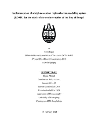
- 28. 21 Chapter Four Implementation and analysis of the ROMS’s Simulated results and Discussions 4.1 Wind circulation The model depicts the annual wind circulation that changes its direction twice a year. The wind circulation is characterized by northeast winds that blow from November to February and southwest winds that blow from May to September with maximum intensity in the center of the Bay of Bengal. The transitional periods from winter to the summer monsoon period is about 105 days and from the summer to the winter period is 285 days. The circulation system in the BoB is very complex that consists of seasonally strong currents with transient eddies superimposed on a background of seasonally changing large-scale gyres. From the model, the northeasterly winds during the winter and southwesterly during the summer flow over the BoB with maximum intensity between 5 to 14o N clockwise wind pattern with maximum intensity along the western boundary of the basin during spring (Figure 12 and 13). And anticlockwise wind circulation in the southern BoB but the clockwise wind circulation in the northern BoB during the autumn prevails over this region. 4.2 General circulation of the Bay of Bengal Because of ocean internal instability, local Ekman pumping, and remote response from the equatorial Indian ocean current, The circulations in the BoB(BoB) are known for eddy-mean flow interactions driven by the strong East Indian coastal current (EICC) and spatial gradient in the density distribution. Owing to the westward propagation of mesoscale eddies embedded within the large-scale planetary Rossby wave, circulation in the western part of the BoB is strongly dominated by eddy mean flow interaction compared to the eastern part. In fact, intense eddies activities prevailed in the entire BoB during all dominant seasons viz., winter (October- January), summer (June to September), and spring (February-May). The surface circulation is characterized by mainly the intense and narrow EICC which flows northward along the southern part of the east coast of India and southward along the northern part. The northern EICC in the southern part separates from the coast at around 16o N. The interannual variability and the external forcing mechanisms were investigated by several researchers using a numerical model showed that role of seasonal coastal Kelvin waves in the development of the EICC. Cheng et al. (2018) examined the eddy statistics and eddy generation mechanism using satellite data and 1-1/2 layer reduced gravity model to conclude that eddies are mainly generated interpersonal wind, with nonlinear interaction with coastline geometry and bathymetry. The eddies subsequently propagate southwestward with a period of 30-120 days and in the western boundary (Seo et al., 2018, Dandapat et al. 2018).
- 29. 22 Figure 12. Circulation in the entire BoB in three different seasons (spring, summer, and winter) The model outputs showed that Anticyclonic eddies are dominated in the Upper BoB whereas well-established cyclonic eddies are found in the southern portion. A cyclonic gyre that forms in the southwestern BoB during October. In December it covered almost the whole bay from 84ºE to 93ºE and 8ºN to 18ºN. It dies off until late April where we can only see a cyclonic eddy centered at 12ºN 86ºE. At the end of June, the circulation in the Bay is mainly anticyclonic and dominated by four eddies centered at 10ºN 83ºE, 11ºN 86ºE, 15ºN 91ºE1, and 8ºN 86ºE (Figure 12). During July these anticyclonic eddies move towards the west of the bay and by the end of August, the anticyclonic circulation of the Bay is confined to the west of the bay. In September the anticyclonic gyre is much smaller and to the north of the Bay. The upper layer circulation of the BoB is subjected to strong seasonal variability. During the early northeast monsoon in November, the large-scale flow pattern in the bay is cyclonic and the western boundary current, the east Indian coastal current (EICC) flows southward from the Bengal shelf north of 20N to the east coast of Sri Lanka. In February the EICC reverses and flows northward along the Indian coast reaching its maximum strength during the early southwest monsoon in April and May and large-scale flow is anticyclonic. This variability is associated with the Indian monsoon: dry northeasterly winds coupled with cooling and evaporation in winter and southwesterly winds coupled heating, precipitation, and increased freshwater runoff from rivers into the northern bay in summer (Shetye et al., 1993). The western boundary current in the BoB appears to lead the wind field and the EICC flows against the local winds at the end of the monsoon seasons. This unusual and complex pattern lead various researchers to consider the role of the remote forcing effects such as Ekman pumping during the height of the respective monsoon seasons, leading to a Sverdrup type circulations that are closed through the coastal current at the western boundary, planetary waves originating at the
- 30. 23 eastern boundary through the radiation of the coastal Kelvin wave energy, planetary waves generated at the eastern boundary through fluctuations of the western boundary current and the monsoon winds can thus be explained by the time the planetary wave takes to cross the BoB(Eigenheer & Quadfasel, 2000). Figure 13. Movement of surface current in three different seasons Here, A denotes surface current during the spring monsoon, B denotes summer and C represents surface current during the winter monsoon. 4.3 Movement of Temperature and salt It is well known that freshwater discharge has a direct impact on sea surface salinity (SSS). The Ganges-Brahmaputra-Meghna and Irrawaddy are the major freshwater contributors that flow into the Bay of Bengal, reaches peaks in June-October. The river discharge into the bay increases and freshwater starts to accumulate in the northern bay with the initiation of southwest monsoon over the Indian peninsula in June (Figure 14). The low salinity water is trapped at the surface due to its hydrostatic property and is pushed offshore by surface Ekman flow. As a consequence, SSS in the northern BoB decreases from June (Fig. 6). The low saline water spreads slowly towards the south and the interior parts of the bay in subsequent months driven by ocean circulation. The SSS in the BoB attains its minimum value during October. Researchers also found in the case of vertical movement of salinity in the BoB that lower surface salinities and shallow halocline at 5-20m depth in summer, autumn, and winter. Sea surface salinity is relatively high in the march-may (spring) (Bhat et al., 2001; Sengupta, Bharath Raj, Ravichandran, Sree Lekha, & Papa, 2016; Vinayachandran, Murty, & Ramesh Babu, 2002). The freshwater discharge from rivers and rainfalls is very important during the summer monsoon. The freshwater plume along the northwest part of the Bay is well reproduced by the model even if the river discharge was not included in the model. It does not advect towards the interior of the bay not until the end of the southwest winds.
- 31. 24 The models show the seasonal cycle of the surface temperature. A researcher experimented on the basis of ocean simulation of salinity budget over the BoB using the Hybrid Coordinate Ocean Model (HYCOM) which showed the salinity changes due to surface freshwater fluxes is the single largest driver of upper 30-m salinity variability in the Bay of Bengal. The seasonality of the total freshwater has the largest effect between June and August. HYCOM predicted the water exported out of the bay by EICC is more saline than the water flowing into the bay (Wilson & Riser, 2016). Figure 14.Vertical transects of Salinity 4.4 Comparison of simulations with drifter and Argo data and evaluation The surface circulation for the three months February, June, and October are presented in figure 20. Simulated sea surface temperature profiles are compared with the available Argo mean data profile at some random locations (Figure 15). We can say that model generates much similar vertical temperature for the Bay of Bengal. Chao et. al., 2018 compared ROMS’s simulated data with assimilated data as a consistency check where satellite obtained sea surface temperature and vertical profiles between observation and ROMS nowcasts were mostly less than 0.5o C while salinity to be 0.09 or less.
- 32. 25 Figure 15. The figure of the comparison of the ROMS and Argo data of the temperature
- 33. 26 Chapter Five Conclusion The simple Ocean model for the Bay of Bengal was tried to develop and implement with the help of ROMS. This model resolved some important atmospheric and oceanic features in reasonable ways, analyzed and presented in this research. Nevertheless, the model depicts the seasonal changes especially in the south of the Bay, and the mesoscale features that dominate the region. Finally, different models and different conditions produce different simulations. Some parameters such as temperature and salinity were verified with model and Argo data in the area of the Bay of Bengal. However, The Bay of Bengal has complex and complicated current patterns because of its geography and unique wind forces. Because of a scarcity of in-situ data, lack of previous experience, inefficient coding, and digital storage problems, many small and large scale features are excluded from this model and are not well understood. In order to get a more accurate model result, factors such as freshwater discharge, rainfall, evaporation, equatorial currents, and other local factors must be taken into account. The lack of high resolution bathymetric, forcing data and inefficiency of the developed model suggests a need for coordinated efforts to survey and collected data across the Bay on a regular basis as well as highly-trained technical persons in the future.
- 34. 27 Chapter Six References Amol, P., Vinayachandran, P. N., Shankar, D., Thushara, V., Vijith, V., Chatterjee, A., & Kankonkar, A. (2019). Effect of freshwater advection and winds on the vertical structure of chlorophyll in the northern Bay of Bengal. Deep-Sea Research Part II: Topical Studies in Oceanography. https://doi.org/https://doi.org/10.1016/j.dsr2.2019.07.010 Antony, C., & Unnikrishnan, A. S. (2013). Observed characteristics of tide-surge interaction along the east coast of India and the head of the Bay of Bengal. Estuarine, Coastal and Shelf Science, 131, 6– 11. https://doi.org/https://doi.org/10.1016/j.ecss.2013.08.004 Bharathi, M. D., Sarma, V., Ramaneswari, K., & Venkataramana, V. (2018). Influence of river discharge on abundance and composition of phytoplankton in the western coastal Bay of Bengal during peak discharge period. Marine Pollution Bulletin, 133, 671–683. Bhardwaj, P., Singh, O., Pattanaik, D. R., & Klotzbach, P. J. (2019). Modulation of bay of bengal tropical cyclone activity by the madden-julian oscillation. Atmospheric Research. Bhat, G. S., Gadgil, S., Hareesh Kumar, P. V, Kalsi, S. R., Madhusoodanan, P., Murty, V. S. N., … others. (2001). BOBMEX: The Bay of Bengal monsoon experiment. Bulletin of the American Meteorological Society, 82(10), 2217–2244. Cane, M. A. (1986). Introduction to Ocean Modeling. Advanced Physical Oceanographic Numerical Modelling, 5–21. https://doi.org/10.1007/978-94-017-0627-8_2 Canuto, V.M., A. Howard, Y. Cheng, M.S. Dubovikov, 2001: Ocean turbulence I: one-point closure model. Momentum and heat vertical diffusivities. J. Phys. Oceanogr. 31, 1413-1426. Chakraborty, A., & Gangopadhyay, A. (2015). Development of a high-resolution multiscale modeling and prediction system for Bay of Bengal, Part I: Climatology-based simulations. Open Journal of Marine Science, 6(1), 145–176. Cheng, X., McCreary, J. P., Qiu, B., Qi, Y., Du, Y., & Chen, X. (2018). Dynamics of eddy generation in the central Bay of Bengal. Journal of Geophysical Research: Oceans, 123(9), 6861-6875. Chao, Y., Farrara, J. D., Zhang, H., Armenta, K. J., Centurioni, L., Chavez, F., ... & Walter, R. K. (2018). Development, implementation, and validation of a California coastal ocean modeling, data assimilation, and forecasting system. Deep Sea Research Part II: Topical Studies in Oceanography, 151, 49-63. Coleman, J. M. (1969). Brahmaputra River: channel processes and sedimentation. Sedimentary Geology, 3(2–3), 129–239. Costa, T. C., Pereira, L. T., Marta-Almeida, M., & Guedes Soares, C. (2018). Mapping of currents off the northwestern Iberian coast with the Regional Ocean Modelling System. Journal of Operational Oceanography, 1–13. doi:10.1080/1755876x.2018.1522717 Dandapat, S., Chakraborty, A., & Kuttippurath, J. (2018). Interannual variability and characteristics of the East India Coastal Current associated with Indian Ocean Dipole events using a high resolution
- 35. 28 regional ocean model. Ocean Dynamics, 68(10), 1321-1334. Demers, S., Legendre, L., & Therriault, J.-C. (1986). Phytoplankton responses to vertical tidal mixing. In Tidal mixing and plankton dynamics (pp. 1–40). Springer. Dey, S. P., Dash, M. K., Sasmal, K., Jana, S., & Raju, N. J. (2020). Impact of river runoff on seasonal sea level, Kelvin waves, and East India Coastal Current in the Bay of Bengal: A numerical study using ROMS. Regional Studies in Marine Science, 35, 101214. Dinesh Kumar, P. K., Paul, Y. S., Muraleedharan, K. R., Murty, V. S. N., & Preenu, P. N. (2016). Comparison of long-term variability of Sea Surface Temperature in the Arabian Sea and Bay of Bengal. Regional Studies in Marine Science, 3, 67–75. https://doi.org/https://doi.org/10.1016/j.rsma.2015.05.004 Eigenheer, A., & Quadfasel, D. (2000). Seasonal variability of the Bay of Bengal circulation inferred from TOPEX/Poseidon altimetry. Journal of Geophysical Research: Oceans, 105(C2), 3243–3252. Ezer, T., & Mellor, G. L. (1997). Simulations of the Atlantic Ocean with a free surface sigma coordinate ocean model. Journal of Geophysical Research: Oceans, 102(C7), 15647-15657. Fairall, C. W., Bradley, E. F., Rogers, D. P., Edson, J. B., & Young, G. S. (1996). Bulk parameterization of air-sea fluxes for tropical ocean-global atmosphere coupled-ocean atmosphere response experiment. Journal of Geophysical Research: Oceans, 101(C2), 3747–3764. Goodbred, S. L., & Saito, Y. (2012). Tide-dominated deltas. In Principles of tidal sedimentology (pp. 129–149). Springer. Griffies, S. M., & Treguier, A. M. (2013). Ocean circulation models and modeling. International Geophysics, 103, 521–551. https://doi.org/10.1016/B978-0-12-391851-2.00020-9 Haas, K. A., & Warner, J. C. (2009). Comparing a quasi-3D to a full 3D nearshore circulation model: SHORECIRC and ROMS. Ocean Modelling, 26(1–2), 91–103. Haidvogel, D. B., Arango, H. G., Hedstrom, K., Beckmann, A., Malanotte-Rizzoli, P., & Shchepetkin, A. F. (2000). Model evaluation experiments in the North Atlantic Basin: Simulations in nonlinear terrain-following coordinates. Dynamics of Atmospheres and Oceans, 32(3–4), 239–281. https://doi.org/10.1016/S0377-0265(00)00049-X Haidvogel, D. B., & Beckmann, A. (1999). Numerical ocean circulation modeling. World Scientific. Haidvogel, D. B. and A. Beckmann, 1999: Numerical Ocean Circulation Modeling. Imperial College Press. Hill, C., DeLuca, C., Suarez, M., Da Silva, A., & others. (2004). The architecture of the earth system modeling framework. Computing in Science & Engineering, 6(1), 18. Howden, S. D., & Murtugudde, R. (2001). Effects of river inputs into the Bay of Bengal. Journal of Geophysical Research: Oceans, 106(C9), 19825–19843. Janes, S. K. C. (2018). Marine Dynamics and Productivity in the Bay of Bengal. https://doi.org/10.1007/978-3-319-71093-8_14 Killworth, P. D., Webb, D. J., Stainforth, D., & Paterson, S. M. (1991). The development of a free-surface Bryan--Cox--Semtner ocean model. Journal of Physical Oceanography, 21(9), 1333–1348. Kossin, J. P. (2018). A global slowdown of tropical-cyclone translation speed. Nature, 558(7708), 104.
- 36. 29 Kourafalou, V. H., De Mey, P., Le Hénaff, M., Charria, G., Edwards, C. A., He, R., … Zhu, X. (2015). Coastal ocean forecasting: System integration and evaluation. Journal of Operational Oceanography, 8, s127–s146. https://doi.org/10.1080/1755876X.2015.1022336 Kripalani, R. H., & Kumar, P. (2004). Northeast monsoon rainfall variability over south peninsular India vis-à-vis the Indian Ocean dipole mode. International Journal of Climatology: A Journal of the Royal Meteorological Society, 24(10), 1267–1282. Krishna, M. S., Prasad, M. H. K., Rao, D. B., Viswanadham, R., Sarma, V., & Reddy, N. P. C. (2016). Export of dissolved inorganic nutrients to the northern Indian Ocean from the Indian monsoonal rivers during discharge period. Geochimica et Cosmochimica Acta, 172, 430–443. Large, W. G., J. C. McWilliams, and S. C. Doney, 1994: Oceanic vertical mixing: a review and a model with a nonlocal boundary layer parameterization. Rev. Geophys., 32, 363-403. Madhu, N. V, Jyothibabu, R., Maheswaran, P. A., John Gerson, V., Gopalakrishnan, T. C., & Nair, K. K. C. (2006). Lack of seasonality in phytoplankton standing stock (chlorophyll a) and production in the western Bay of Bengal. Continental Shelf Research, 26(16), 1868–1883. https://doi.org/https://doi.org/10.1016/j.csr.2006.06.004 Madhupratap, S. P. K. P. M. M. T. G. P. M. G. N. R. S. N. de S. S. S. M. (2002). Why is the Bay of Bengal less productive during summer monsoon compared to the Arabian Sea? GEOPHYSICAL RESEARCH LETTERS, 29(24), 88-1-88–4. https://doi.org//10.1029/2002GL016013 Maria, A. (2012). Ocean Circulation Modeling : The Bay of Bengal. Retrieved from https://people.mio.osupytheas.fr/~doglioli/Rammou_rapport.pdf Mellor, G. L. and T. Yamada, 1982: Developement of a turbulence closure model for geophysical fluid problems. Rev. Geophys. Space Phys., 20, 851-875. Milliman, J.D. and Meade, R. . (1983). World-Wide Delivery of River Sediment to the Oceans. Journal of Geology, 91, 1–21. https://doi.org/10.1086/628741 Mole, S. (2012). Numerical modelling of tides and storm surges in the Bay of Bengal. Goa University. Nancy Hall. (2015). Navier-Stokes Equations. Retrieved from NASA Official website: https://www.grc.nasa.gov/WWW/k-12/airplane/nseqs.html Nayak, S. R., Sarangi, R. K., & Rajawat, A. S. (2001). Application of IRS-P4 OCM data to study the impact of cyclone on coastal. Current Science, 80(9). Ota, Y., Kuroda, J., Yamaguchi, A., Suzuki, A., Araoka, D., Ishimura, T., … Kawahata, H. (2019). Monsoon-influenced variations in plankton community structure and upper-water column stratification in the western Bay of Bengal during the past 80 ky. Palaeogeography, Palaeoclimatology, Palaeoecology, 521, 138–150. Patra, A., & Bhaskaran, P. K. (2016). Trends in wind-wave climate over the head Bay of Bengal region. International Journal of Climatology, 36(13), 4222–4240. Penven, P., Marchesiello, P., Debreu, L., & Lefèvre, J. (2008). Software tools for pre- and post- processing of oceanic regional simulations. Environmental Modelling and Software, 23(5), 660–662. https://doi.org/10.1016/j.envsoft.2007.07.004 Prakash, K. R., & Pant, V. (2019). On the wave-current interaction during the passage of a tropical cyclone in the Bay of Bengal. Deep Sea Research Part II: Topical Studies in Oceanography, 104658.
- 37. 30 Pramanik, S., Mandal, S., Shee, A., Halder, S., & Sil, S. (2019). Tidal Circulation Studies Using Regional Model in the Bay of Bengal. Proceedings of the Fourth International Conference in Ocean Engineering (ICOE2018), 829–836. Prasanna Kumar, S., Nuncio, M., Narvekar, J., Kumar, A., Sardesai, de S., De Souza, S. N., … Madhupratap, M. (2004). Are eddies nature’s trigger to enhance biological productivity in the Bay of Bengal? Geophysical Research Letters, 31(7). Rahman, M. H. (2007). Legal regime of marine environment in the Bay of Bengal. Atlantic Publishers & Dist. Rao, K. H., Smitha, A., & Ali, M. M. (2006). A study on cyclone induced productivity in south-western Bay of Bengal during November-December 2000 using MODIS (SST and chlorophyll-a). Rao, R. R., Kumar, P. V. H., & Mathew, B. (1994). Near-surface heating in the Arabian Sea during the pre-onset regime of MONEX-79. Meteorology and Atmospheric Physics, 53(1–2), 19–31. Ray, R. D. (1999). A global ocean tide model from TOPEX/POSEIDON altimetry: GOT99. 2. National Aeronautics and Space Administration, Goddard Space Flight Center. Riethmüller, R., Colijn, F., Breitbach, G., Krasemann, H. J., Petersen, W., Schroeder, F., & Ziemer, F. (2009, September). COSYNA a German initiative for an integrated coastal observing system. In Proc. of OceanObs' 09 Conference (pp. 1-4). Rogers, K. G., & Goodbred, S. L. (2014). The Sundarbans and Bengal Delta: the world’s largest tidal mangrove and delta system. In Landscapes and Landforms of India (pp. 181–187). Springer. Rogers, K. G., Goodbred, S. L., & Mondal, D. R. (2013). Monsoon sedimentation on the ‘abandoned’ tide-influenced Ganges–Brahmaputra delta plain. Estuarine, Coastal and Shelf Science, 131, 297– 309. https://doi.org/https://doi.org/10.1016/j.ecss.2013.07.014 Saikranthi, K., Radhakrishna, B., Thota, N. R., & Satheesh, S. K. (2019). Differences in the association of sea surface temperature—precipitating systems over the Bay of Bengal and the Arabian Sea during southwest monsoon season. International Journal of Climatology, 39(11), 4305–4312. https://doi.org/10.1002/joc.6074 Saji, N. H., Goswami, B. N., Vinayachandran, P. N., & Yamagata, T. (1999). A dipole mode in the tropical Indian Ocean. Nature, 401(6751), 360. Sandeep, K. K., & Pant, V. (2019). Riverine freshwater plume variability in the Bay of Bengal using wind sensitivity experiments. Deep Sea Research Part II: Topical Studies in Oceanography, 104649. Sarangi, R. K. (2016). Remote sensing observations of ocean surface chlorophyll and temperature with the impact of cyclones and depressions over the Bay of Bengal Water. Marine Geodesy, 39(1), 53– 76. Sen, R., Pandey, S., Dandapat, S., Francis, P. A., & Chakraborty, A. (2020). A numerical study on seasonal transport variability of the North Indian Ocean boundary currents using Regional Ocean Modeling System (ROMS). Journal of Operational Oceanography, 1-20. Sengupta, D., Bharath Raj, G. N., Ravichandran, M., Sree Lekha, J., & Papa, F. (2016). Near-surface salinity and stratification in the north Bay of Bengal from moored observations. Geophysical Research Letters, 43(9), 4448–4456. Seo, H., Xie, S.-P., Murtugudde, R., Jochum, M., & Miller, A. J. (2009). Seasonal effects of Indian Ocean freshwater forcing in a regional coupled model. Journal of Climate, 22(24), 6577–6596.
- 38. 31 Seo, H., Subramanian, A. C., Song, H., & Chowdary, J. S. (2019). Coupled effects of ocean current on wind stress in the Bay of Bengal: Eddy energetics and upper ocean stratification. Deep Sea Research Part II: Topical Studies in Oceanography, 168, 104617. Shchepetkin, A. F., and J. C. McWilliams (1998), Quasi-monotone advection schemes based on explicit locally adaptive dissipation, Monthly Weather Review, 126, 1541-1580. Shchepetkin, A. F., & McWilliams, J. C. (2005). The regional oceanic modeling system (ROMS): A split- explicit, free-surface, topography-following-coordinate oceanic model. Ocean Modelling, 9(4), 347– 404. https://doi.org/10.1016/j.ocemod.2004.08.002 Shenoi, S. S. C., Shankar, D., & Shetye, S. R. (2002). Differences in heat budgets of the near-surface Arabian Sea and Bay of Bengal: Implications for the summer monsoon. Journal of Geophysical Research: Oceans, 107(C6), 1–5. Shetye, S. R., Gouveia, A. D., Shenoi, S. S. C., Sundar, D., Michael, G. S., & Nampoothiri, G. (1993). The western boundary current of the seasonal subtropical gyre in the Bay of Bengal. Journal of Geophysical Research: Oceans, 98(C1), 945–954. Sindhu, B., & Unnikrishnan, A. S. (2013). Characteristics of tides in the Bay of Bengal. Marine Geodesy, 36(4), 377–407. Sridhar, P. N., Ramana, I. V, Ali, M. M., & Veeranarayana, B. (2008). Understanding the suspended sediment dynamics in the coastal waters of the Bay of Bengal using high resolution ocean colour data. Current Science, 1499–1502. Steven, A. D., Baird, M. E., Brinkman, R., Car, N. J., Cox, S. J., Herzfeld, M., ... & Yu, J. (2019). eReefs: An operational information system for managing the Great Barrier Reef. Journal of Operational Oceanography, 12(sup2), S12-S28. Thadathil, P., Gopalakrishna, V. V, Muraleedharan, P. M., Reddy, G. V, Araligidad, N., & Shenoy, S. (2002). Surface layer temperature inversion in the Bay of Bengal. Deep Sea Research Part I: Oceanographic Research Papers, 49(10), 1801–1818. Thushara, V., & Vinayachandran, P. N. (2016). Formation of summer phytoplankton bloom in the northwestern B ay of B engal in a coupled physical-ecosystem model. Journal of Geophysical Research: Oceans, 121(12), 8535–8550. Thyng, K. M., Kobashi, D., Ruiz-Xomchuk, V., Qu, L., Chen, X., & Hetland, R. D. (2021). Performance of offline passive tracer advection in the Regional Ocean Modeling System (ROMS; v3. 6, revision 904). Geoscientific Model Development, 14(1), 391-407. Tripathy, G.R.; Singh, S.K.; Bhushan, R.; Ramaswamy, V. (2011). Sr–Nd isotope composition of the Bay of Bengal sediments: Impact of climate on erosion in the Himalaya. Geochemical Journal, 45, 175– 186. https://doi.org/10.2343/geochemj.1.0112 Umlauf, L., H. Burchard, 2003: A generic length-scale equation for geophysical turbulence models. J. MArine Res., 61, 235-265. Vinayachandran, P. N. (2010). Impact of physical processes on the chlorophyll distribution in the Bay of Bengal. American Geophysical Union. Vinayachandran, P. N., & Kurian, J. (2007). Hydrographic observations and model simulation of the Bay of Bengal freshwater plume. Deep Sea Research Part I: Oceanographic Research Papers, 54(4), 471–486.
- 39. 32 Vinayachandran, P. N., & Mathew, S. (2003). Phytoplankton bloom in the Bay of Bengal during the northeast monsoon and its intensification by cyclones. Geophysical Research Letters, 30(11). https://doi.org/10.1029/2002GL016717 Vinayachandran, P. N., Murty, V. S. N., & Ramesh Babu, V. (2002). Observations of barrier layer formation in the Bay of Bengal during summer monsoon. Journal of Geophysical Research: Oceans, 107(C12), SRF--19. Warner, J.C, C.R. Sherwood, H.G. Arango, and R.P. Signell, 2005a: Performance of four Turbulence Closure Methods Implemented using a Generic Length Scale Method. Ocean Modelling, 8, 81-113. Webster, P. J., Moore, A. M., Loschnigg, J. P., & Leben, R. R. (1999). Coupled ocean--atmosphere dynamics in the Indian Ocean during 1997--98. Nature, 401(6751), 356. Wilkin, J. L., Arango, H. G., Haidvogel, D. B., Lichtenwalner, C. S., Glenn, S. M., & Hedström, K. S. (2005). A regional ocean modeling system for the Long-term Ecosystem Observatory. Journal of Geophysical Research: Oceans, 110(6), 1–13. https://doi.org/10.1029/2003JC002218 Wilson-Diaz, D., Mariano, A. J., & Evans, R. H. (2009). On the heat budget of the Arabian Sea. Deep Sea Research Part I: Oceanographic Research Papers, 56(2), 141–165. Wilson, E. A., & Riser, S. C. (2016). An assessment of the seasonal salinity budget for the upper Bay of Bengal. Journal of Physical Oceanography, 46(5), 1361–1376. Zhao, C., Daewel, U., & Schrum, C. (2019). Tidal impacts on primary production in the North Sea. Earth System Dynamics, 10(2), 287–317. Zhang, R. H., Yu, Y., Song, Z., Ren, H. L., Tang, Y., Qiao, F., ... & Wang, L. (2020). A review of progress in coupled ocean-atmosphere model developments for ENSO studies in China. Journal of Oceanology and Limnology, 38(4), 930-961.