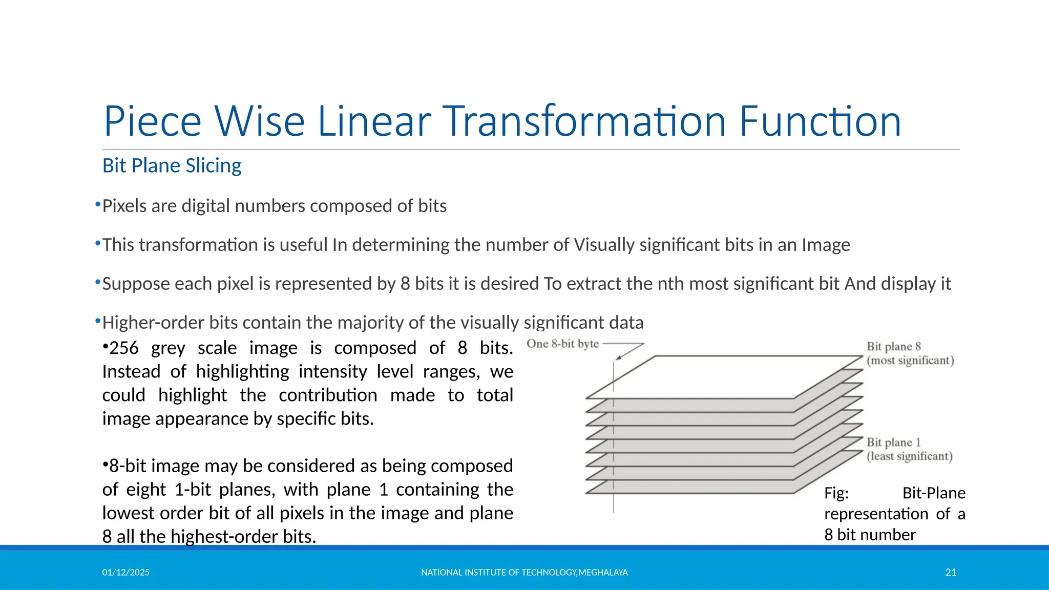
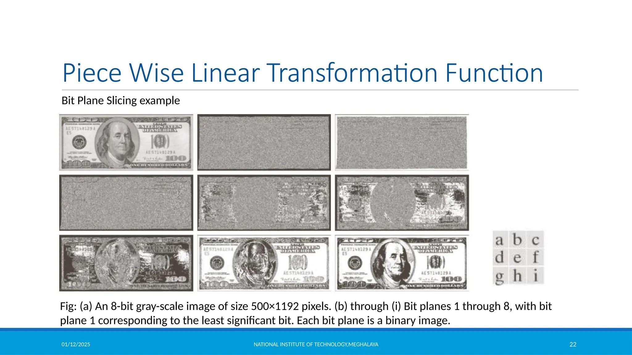
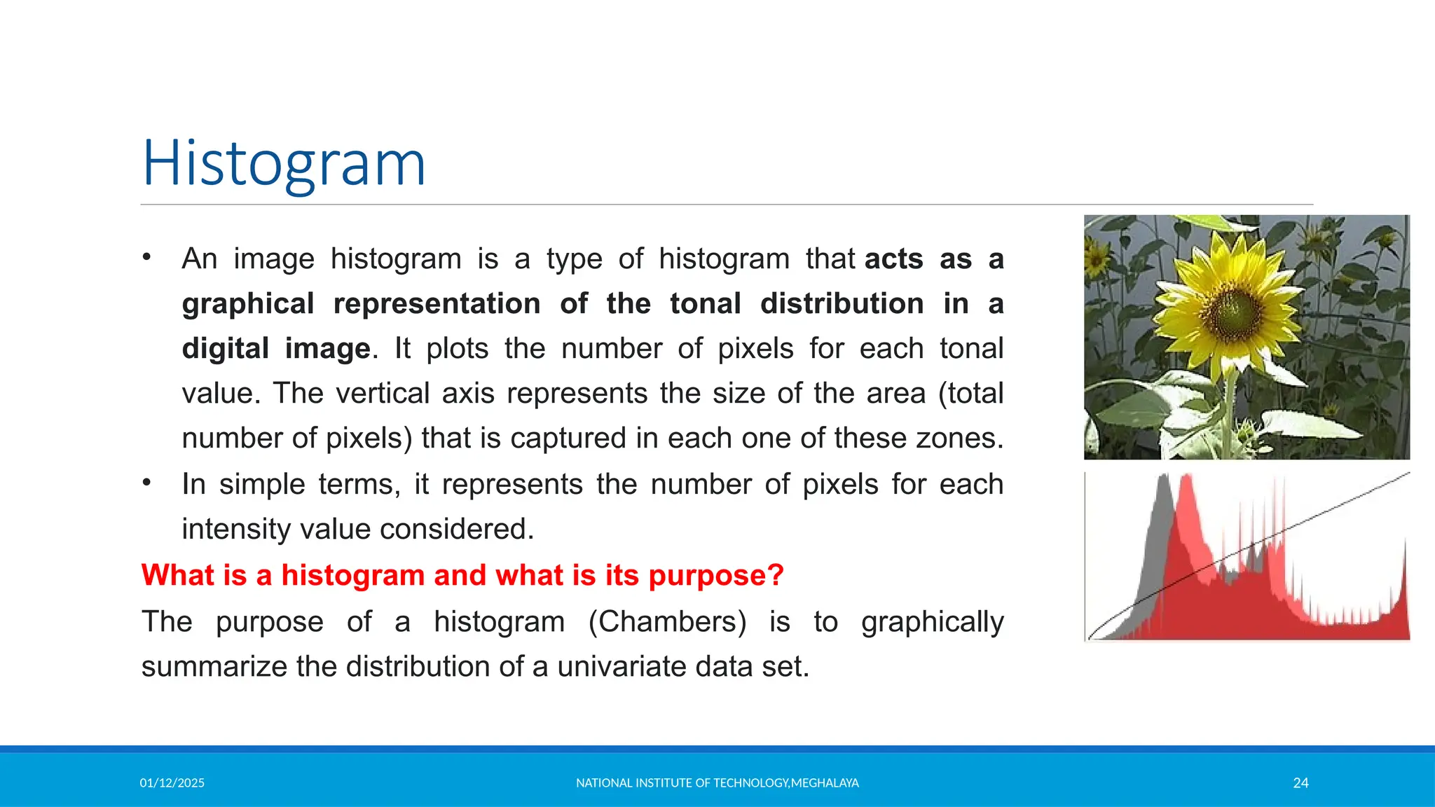
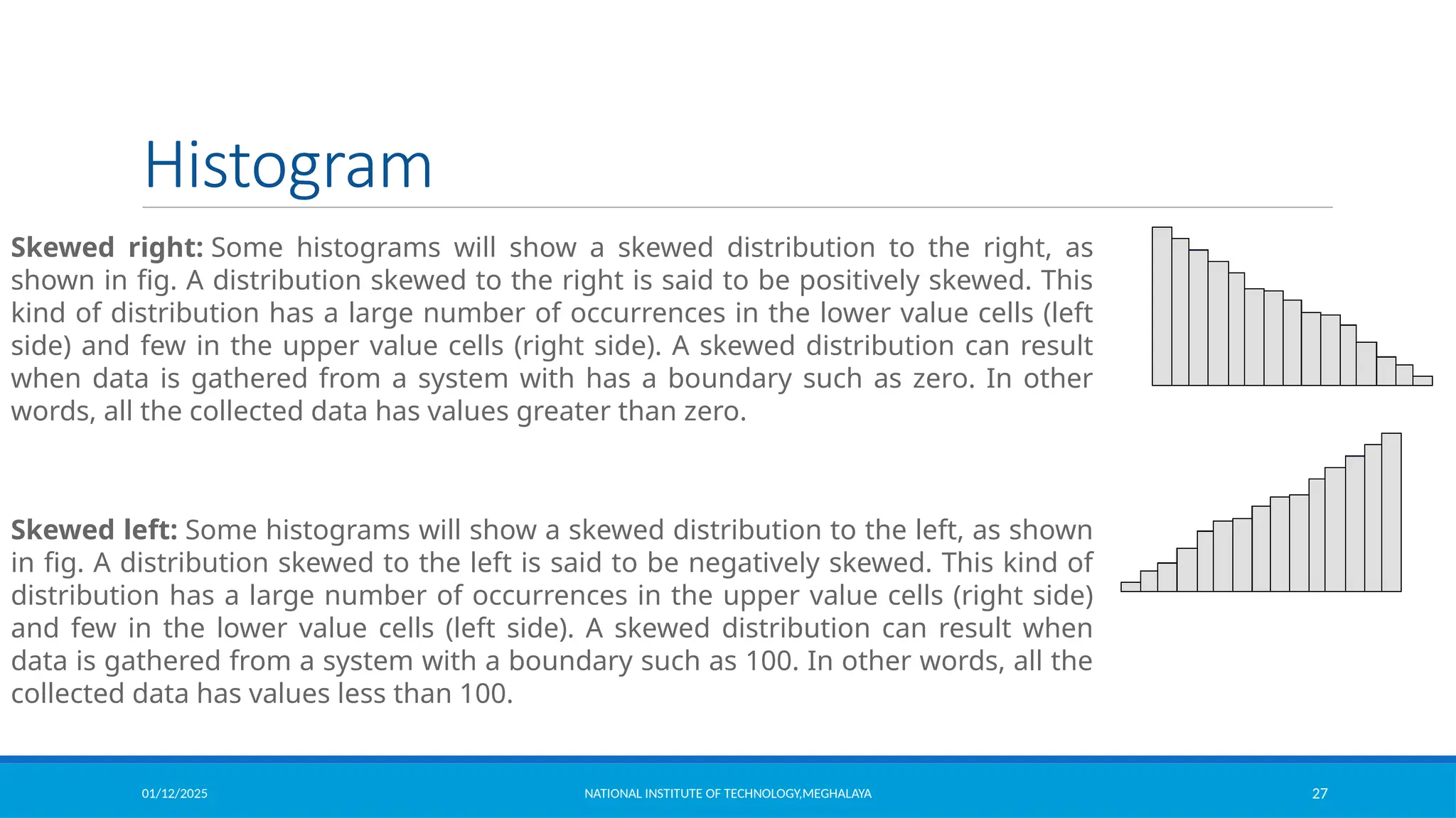
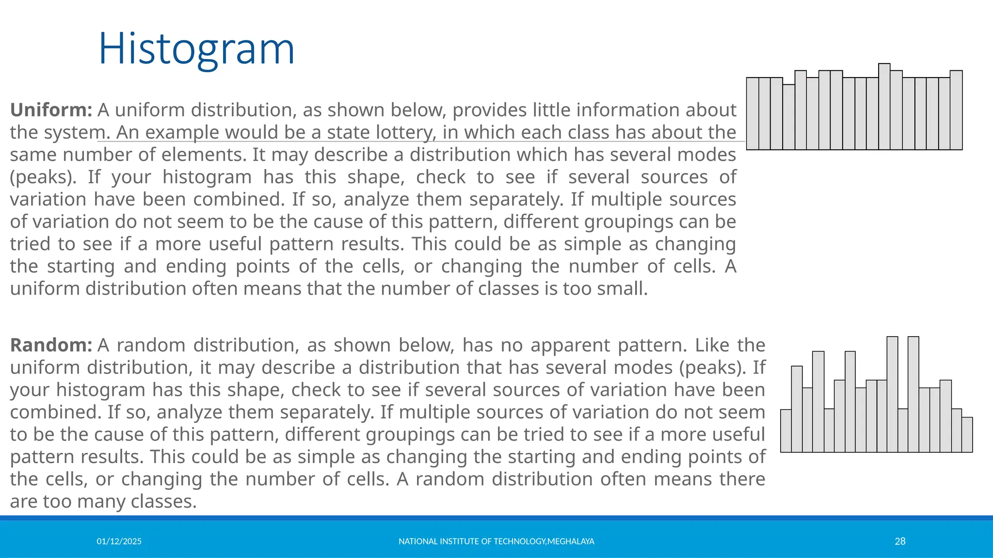
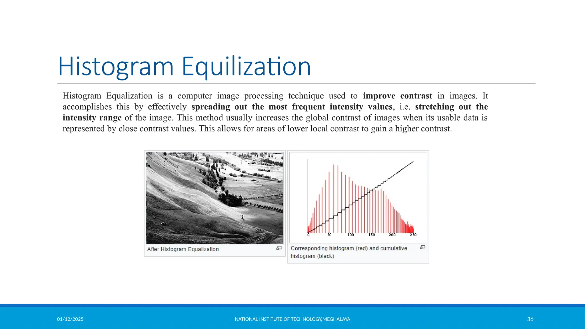
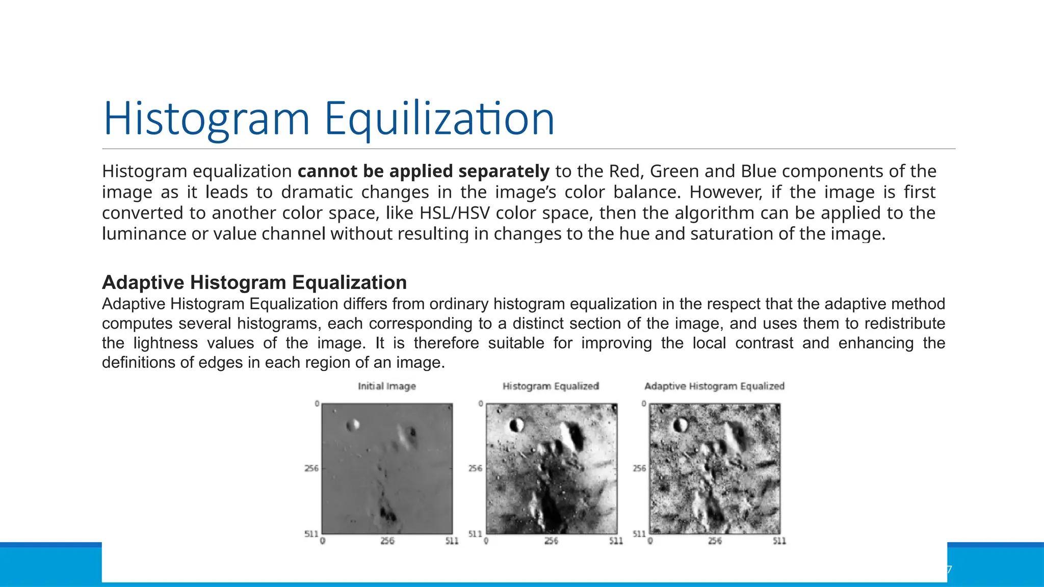
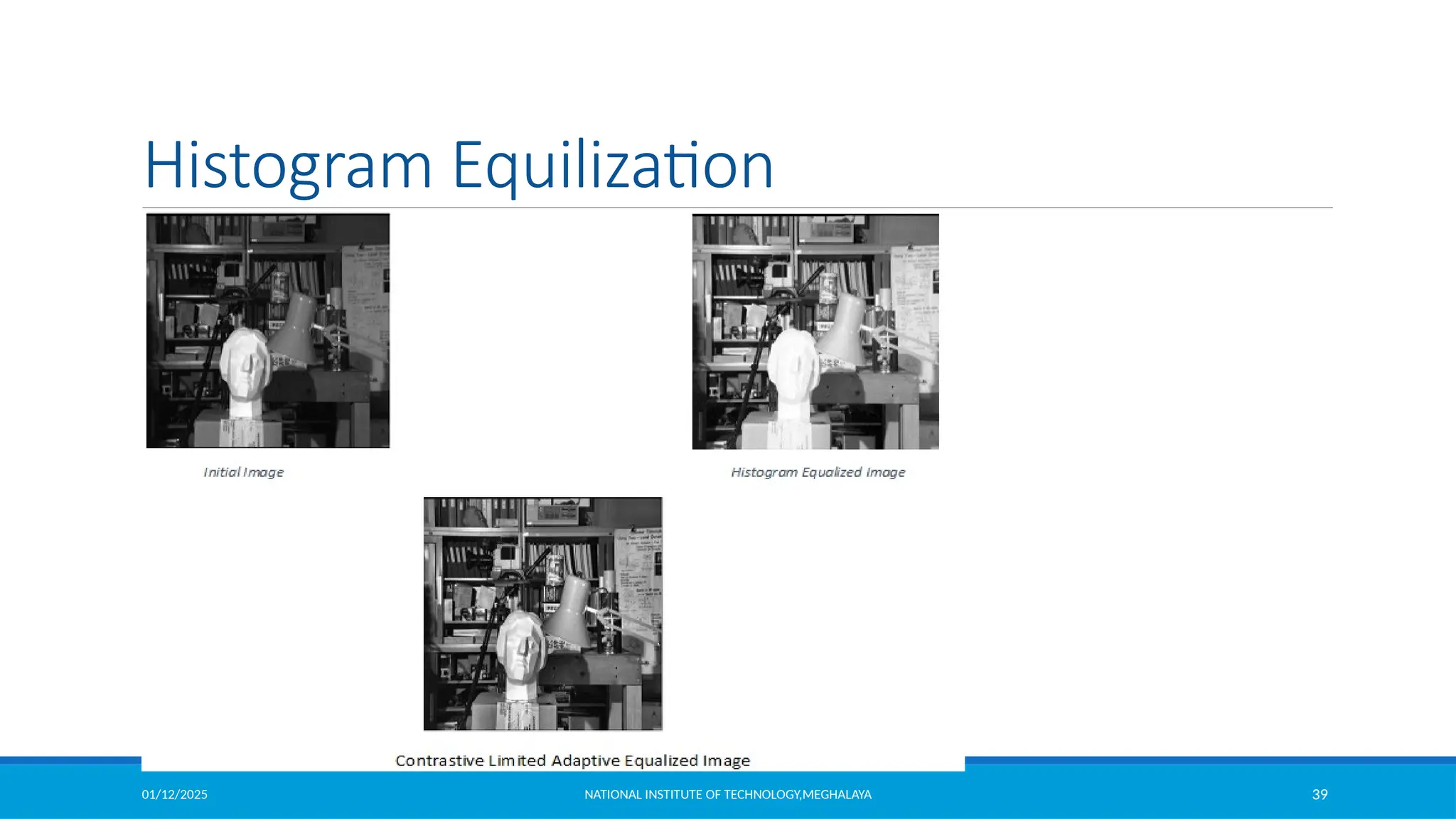
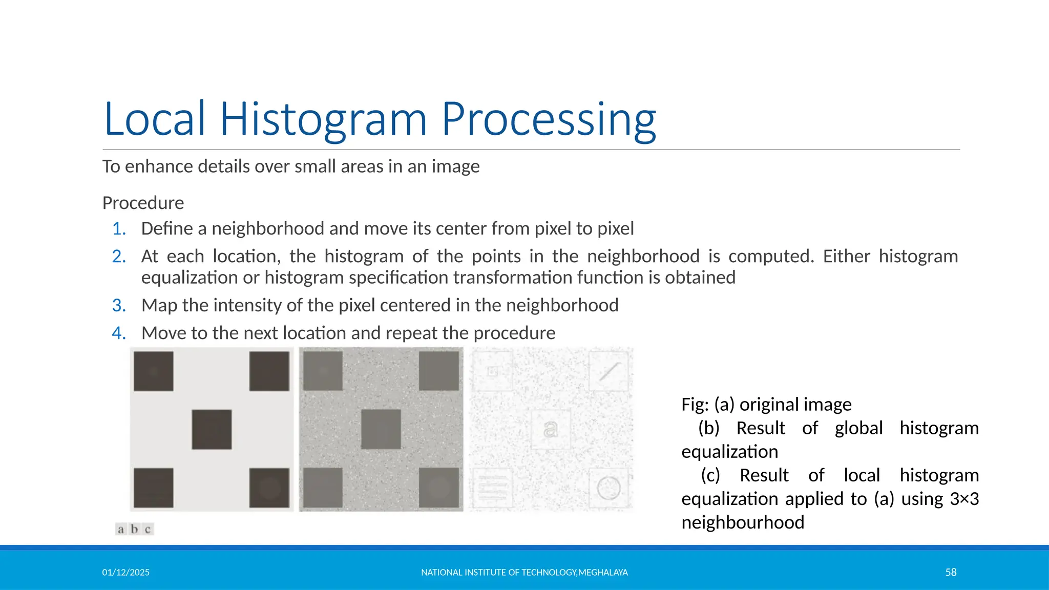
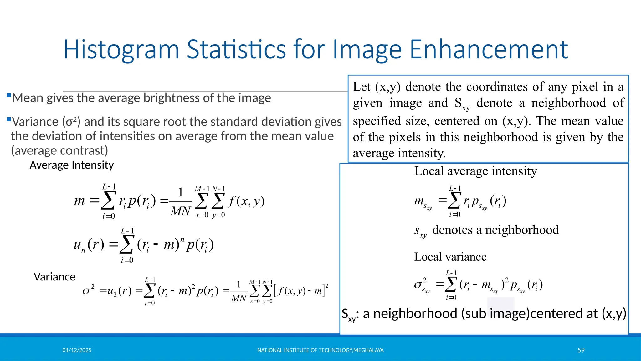
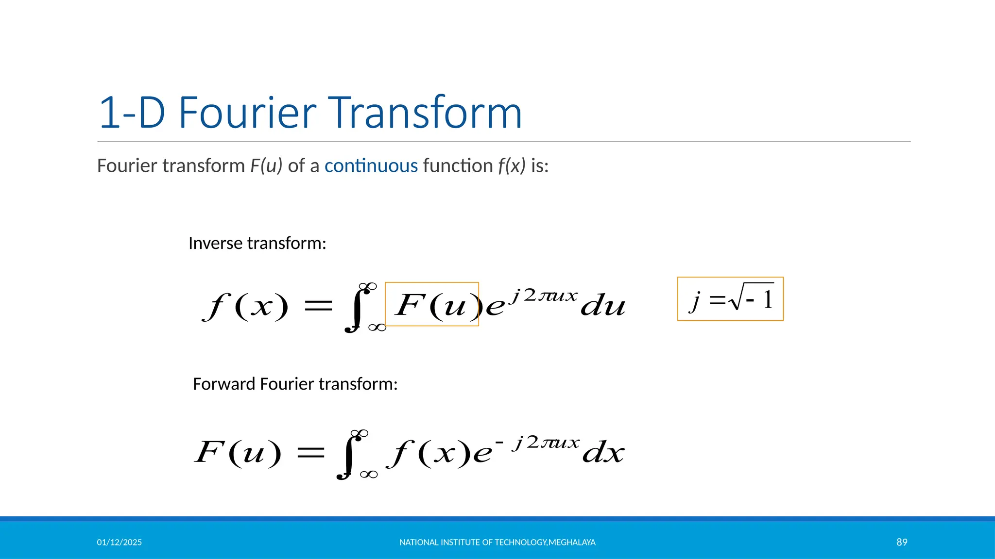
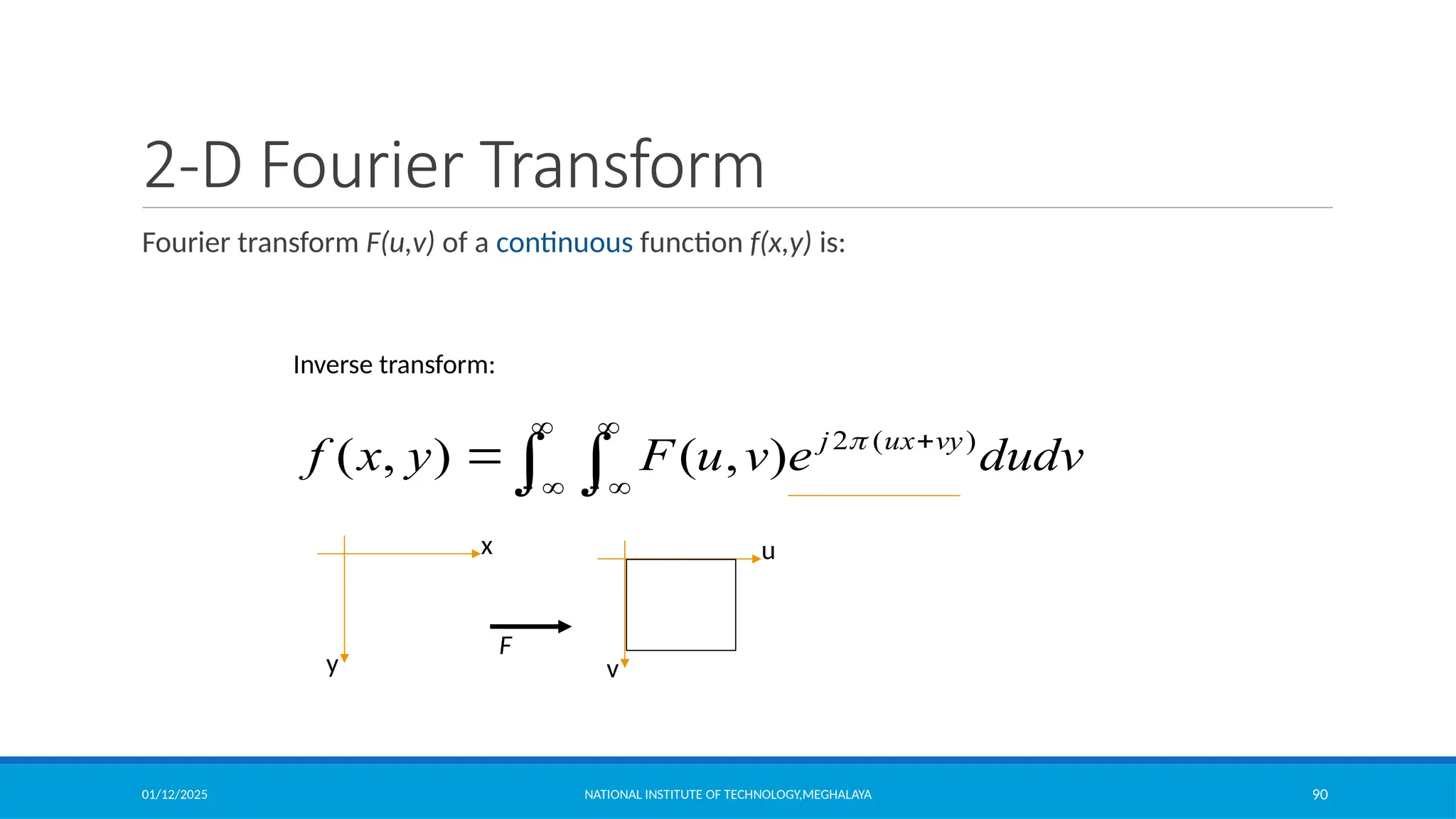
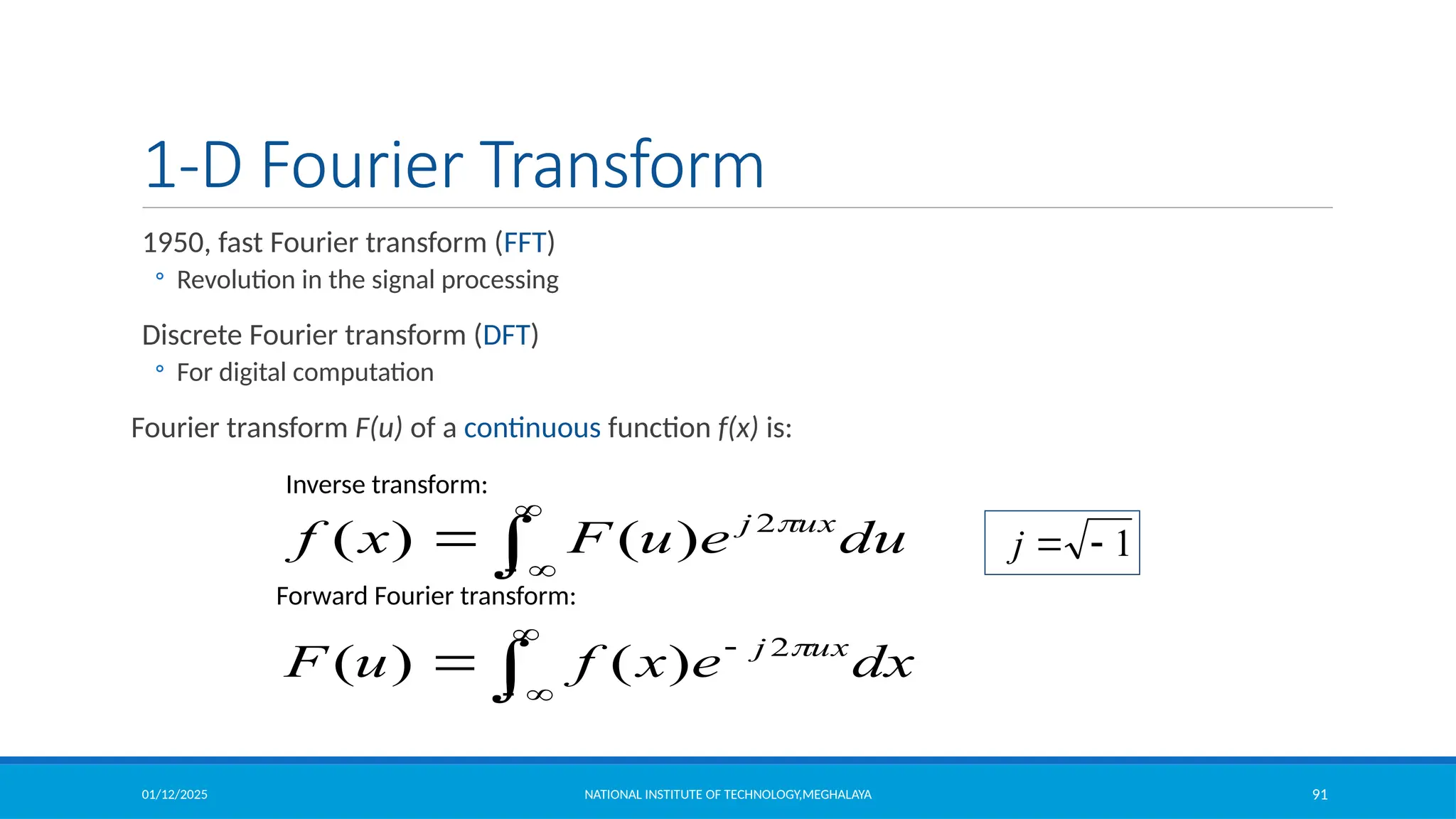
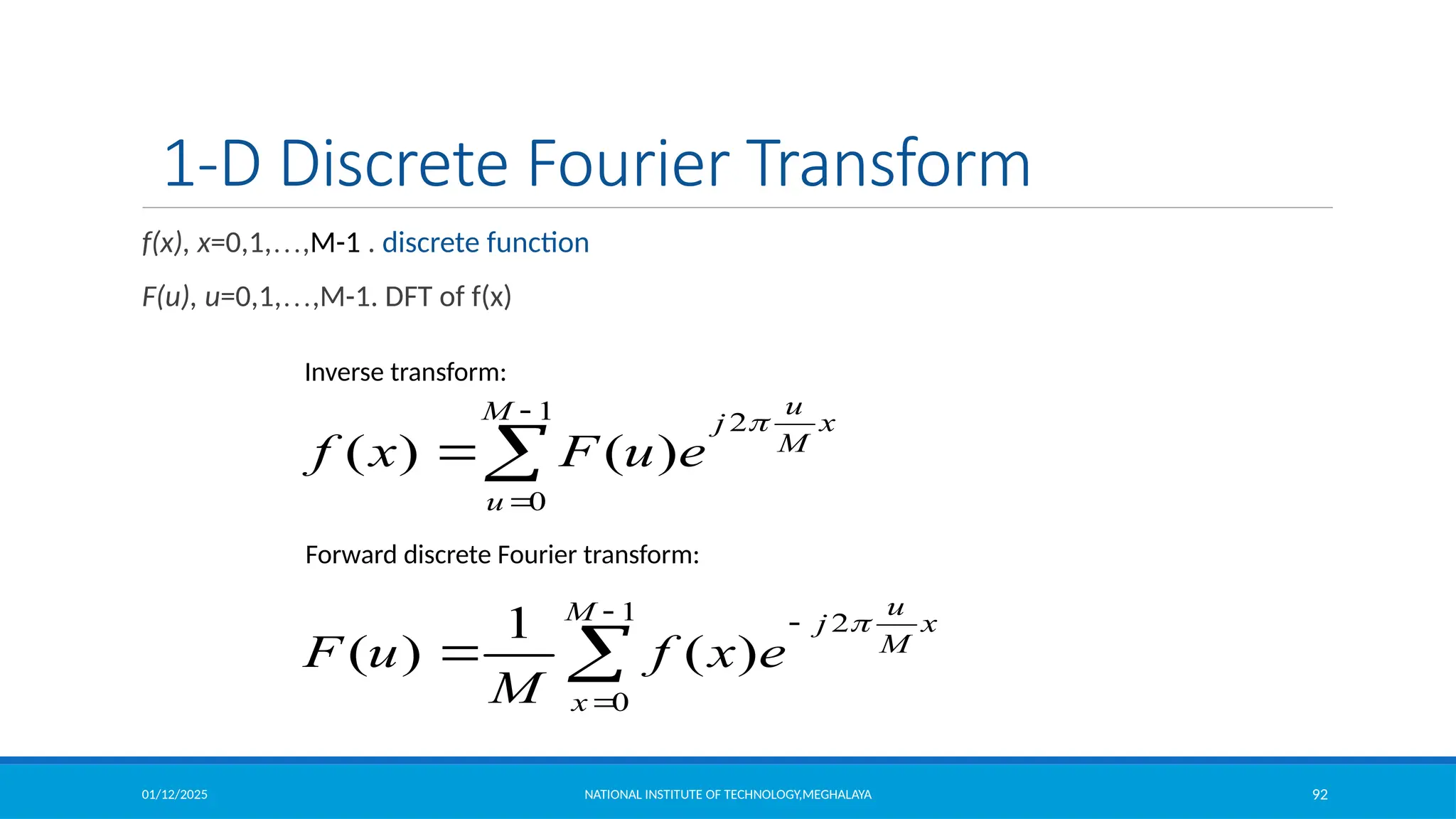
The document outlines image enhancement techniques in both spatial and frequency domains, focusing on methods like grey level transformations, histogram processing, and intensity level slicing. It details various transformations including contrast stretching, logarithmic, and power-law transformations, and emphasizes the importance of histograms in analyzing image tonal distributions. Additionally, it discusses histogram equalization as a method to improve image contrast by redistributing intensity values, with variations like adaptive histogram equalization for localized contrast adjustments.

![01/12/2025 NATIONAL INSTITUTE OF TECHNOLOGY,MEGHALAYA 5
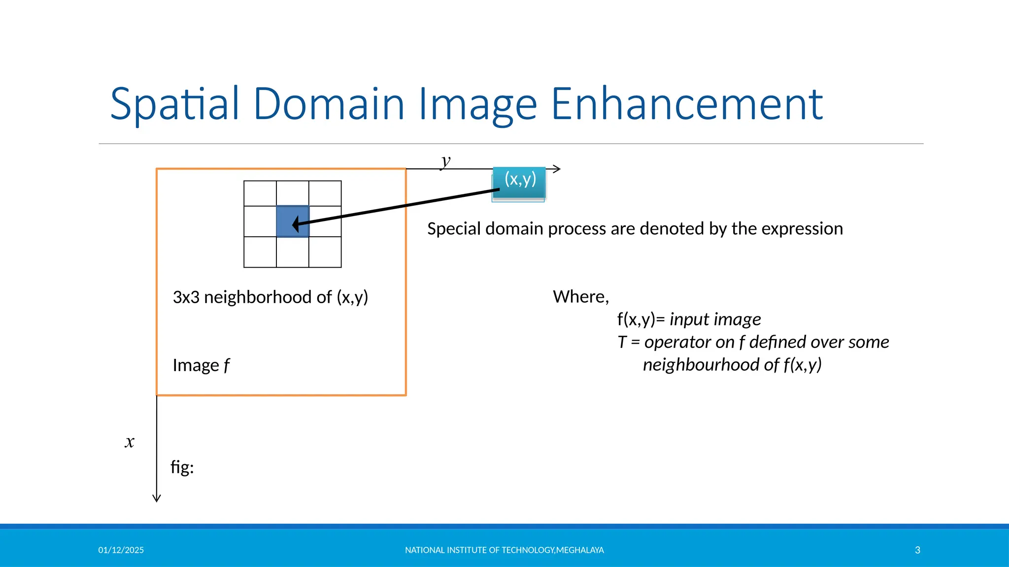
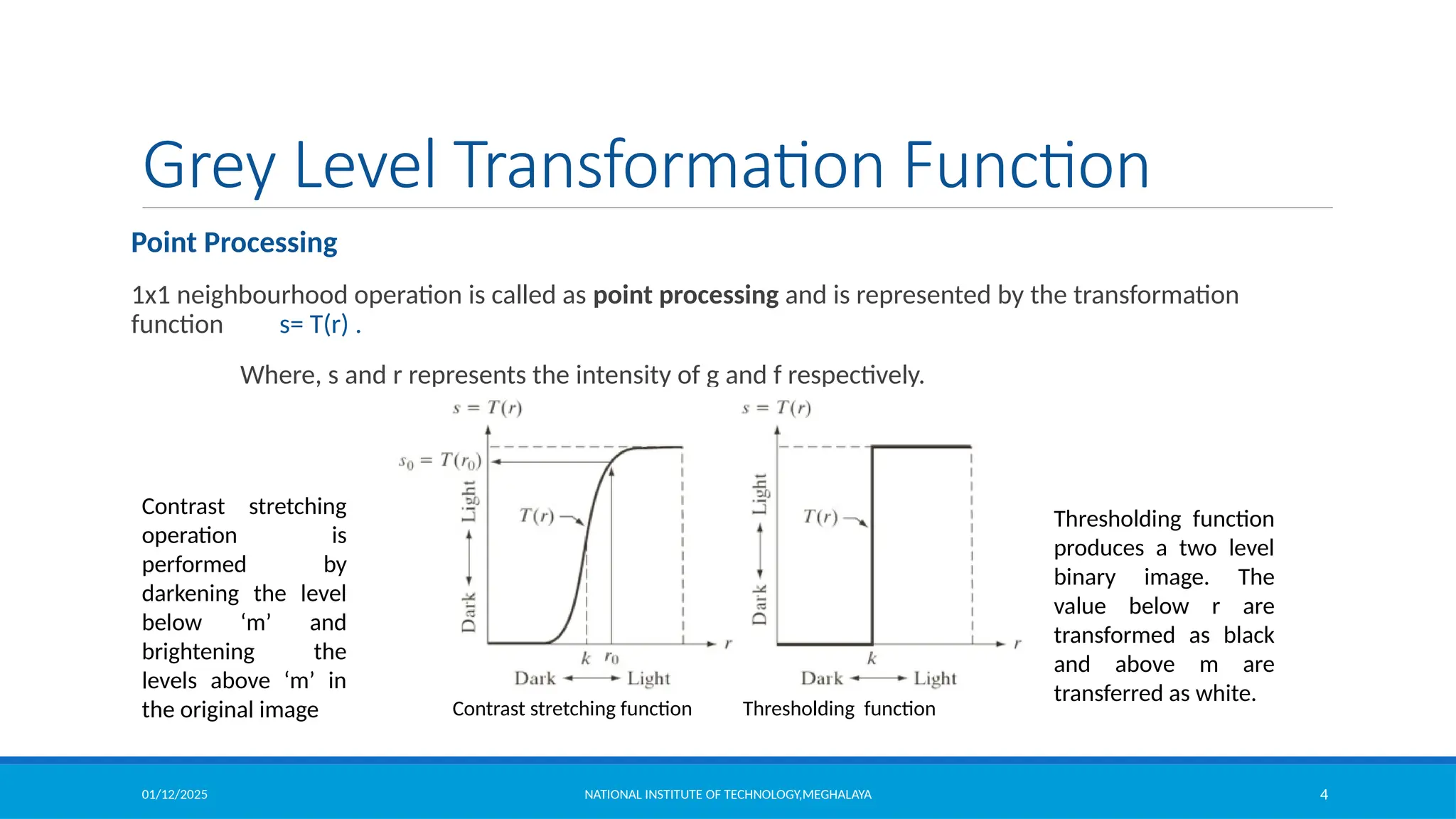
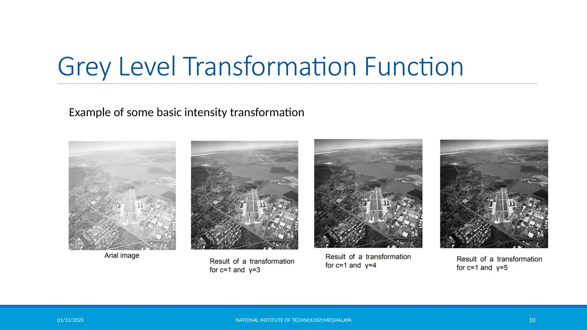
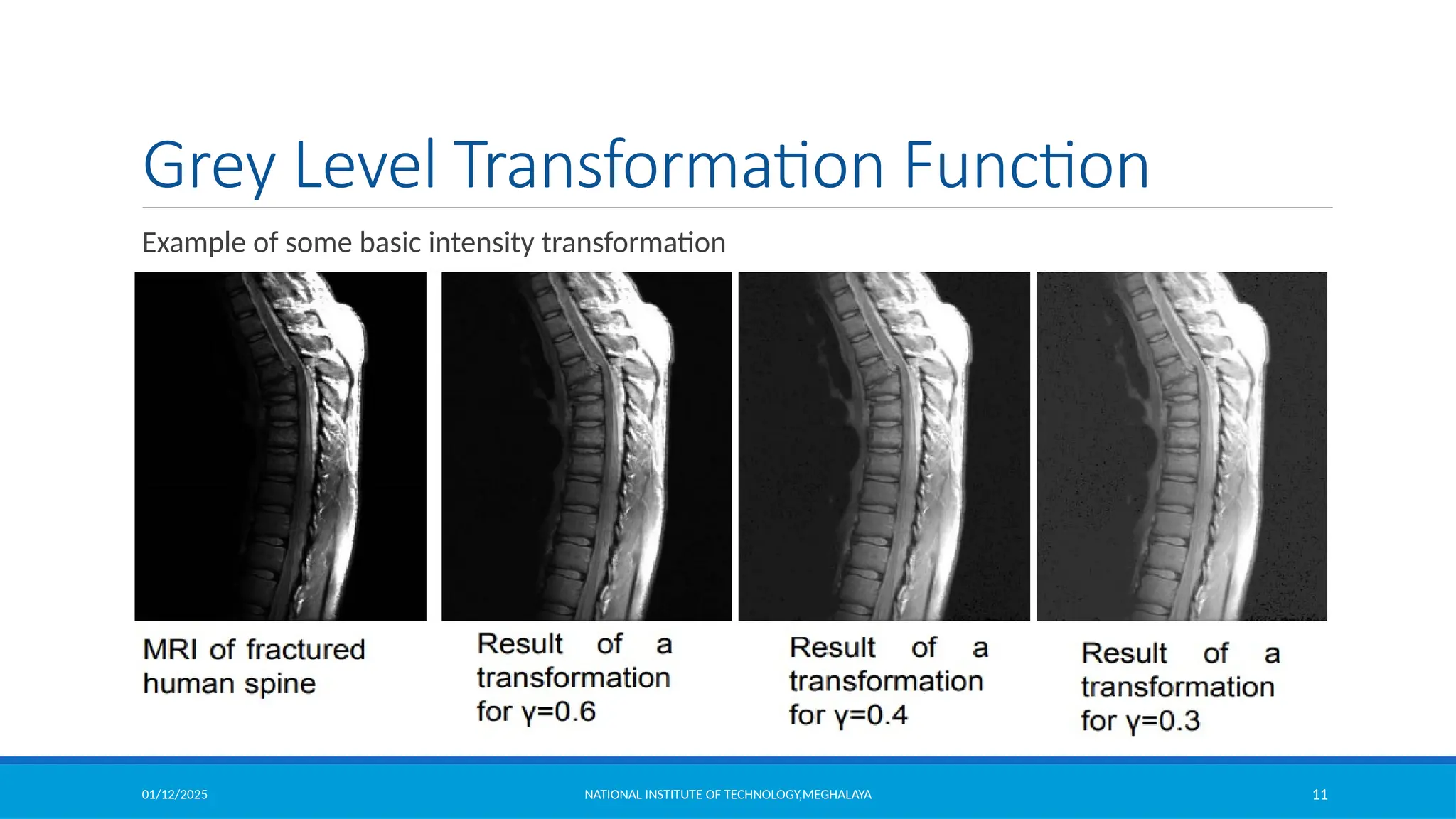
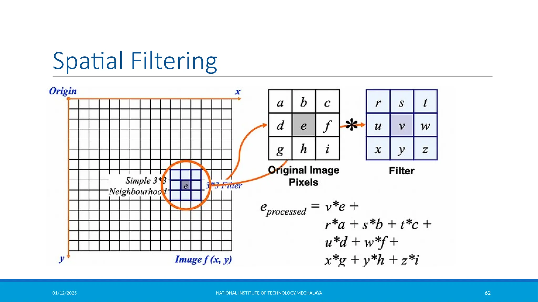
Grey Level Transformation Function
Image negative
Let the image has an intensity level in the range [0 L-1], then the intensity transformation is given by
Where,
S is the output intensity value
L is the highest intensity levels
r is the input intensity value
Particularly suited for
enhancing white or grey detail
embedded in dark regions of an
image, especially when the
black areas are dominant in size](https://image.slidesharecdn.com/module2-250112143149-8855b5c3/75/Image-Enhancement-in-Spatial-Domain-and-Frequency-Domain-5-2048.jpg)
![01/12/2025 NATIONAL INSTITUTE OF TECHNOLOGY,MEGHALAYA 6
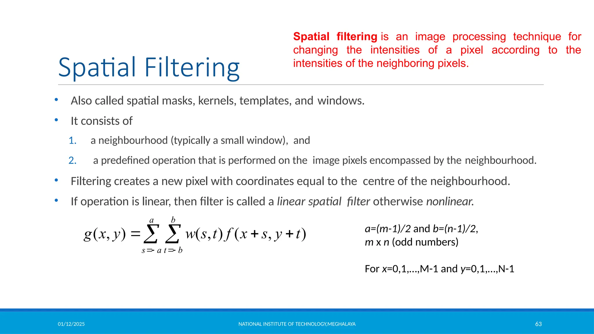
Grey Level Transformation Function
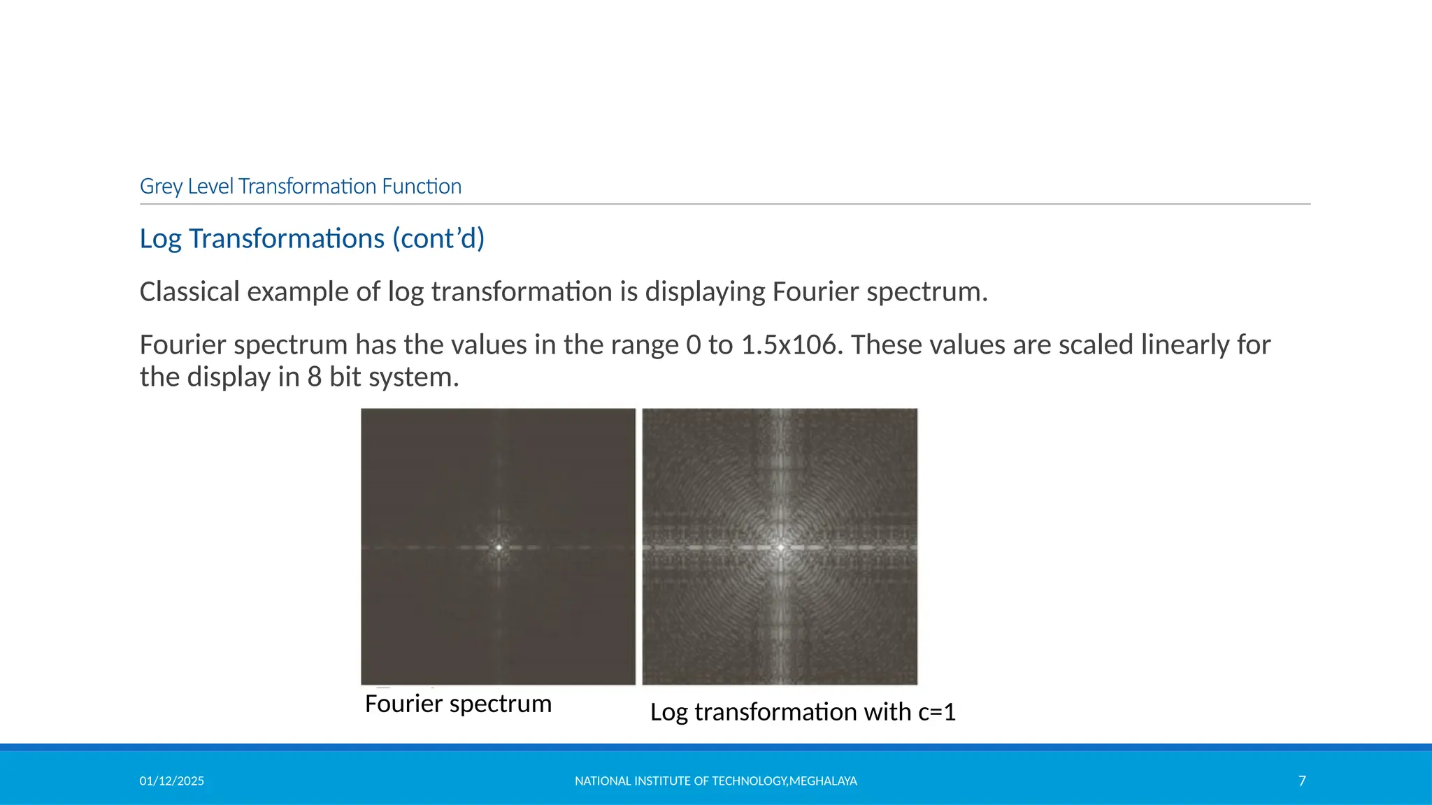
Log Transformations
For an image having intensity ranging from [0 L-1], log transformation is given by
, where c is a constant
• log transformation compresses
the dynamic range of images with
large variations in pixel values.
• It maps a narrow range of low
intensity values in the input into a
wide range of output levels.
• The opposite is true of higher
values of input levels.
• It expands the values of dark
pixels in an image while
compressing the higher level
values.](https://image.slidesharecdn.com/module2-250112143149-8855b5c3/75/Image-Enhancement-in-Spatial-Domain-and-Frequency-Domain-6-2048.jpg)
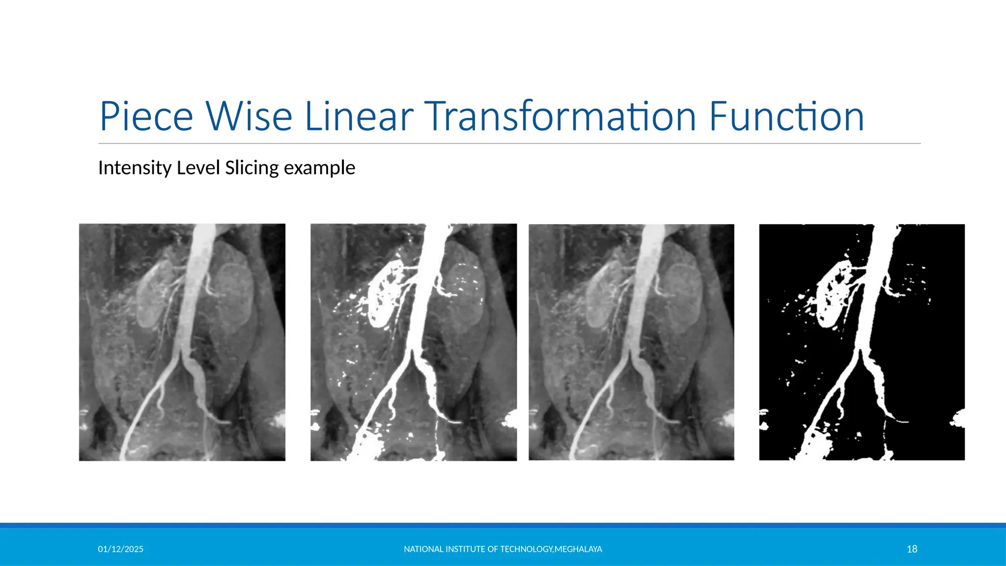
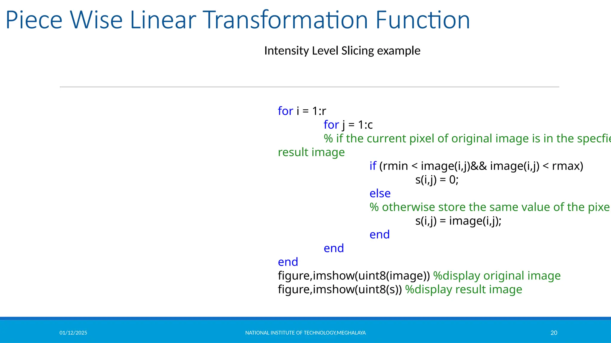
![01/12/2025 NATIONAL INSTITUTE OF TECHNOLOGY,MEGHALAYA 19
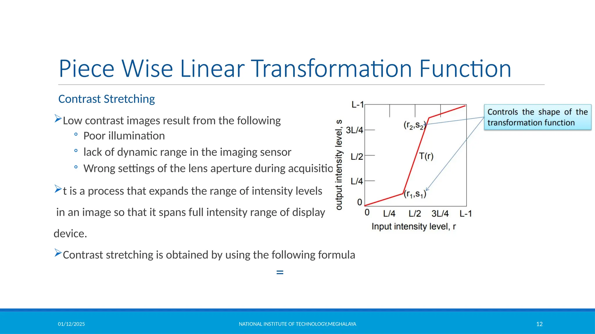
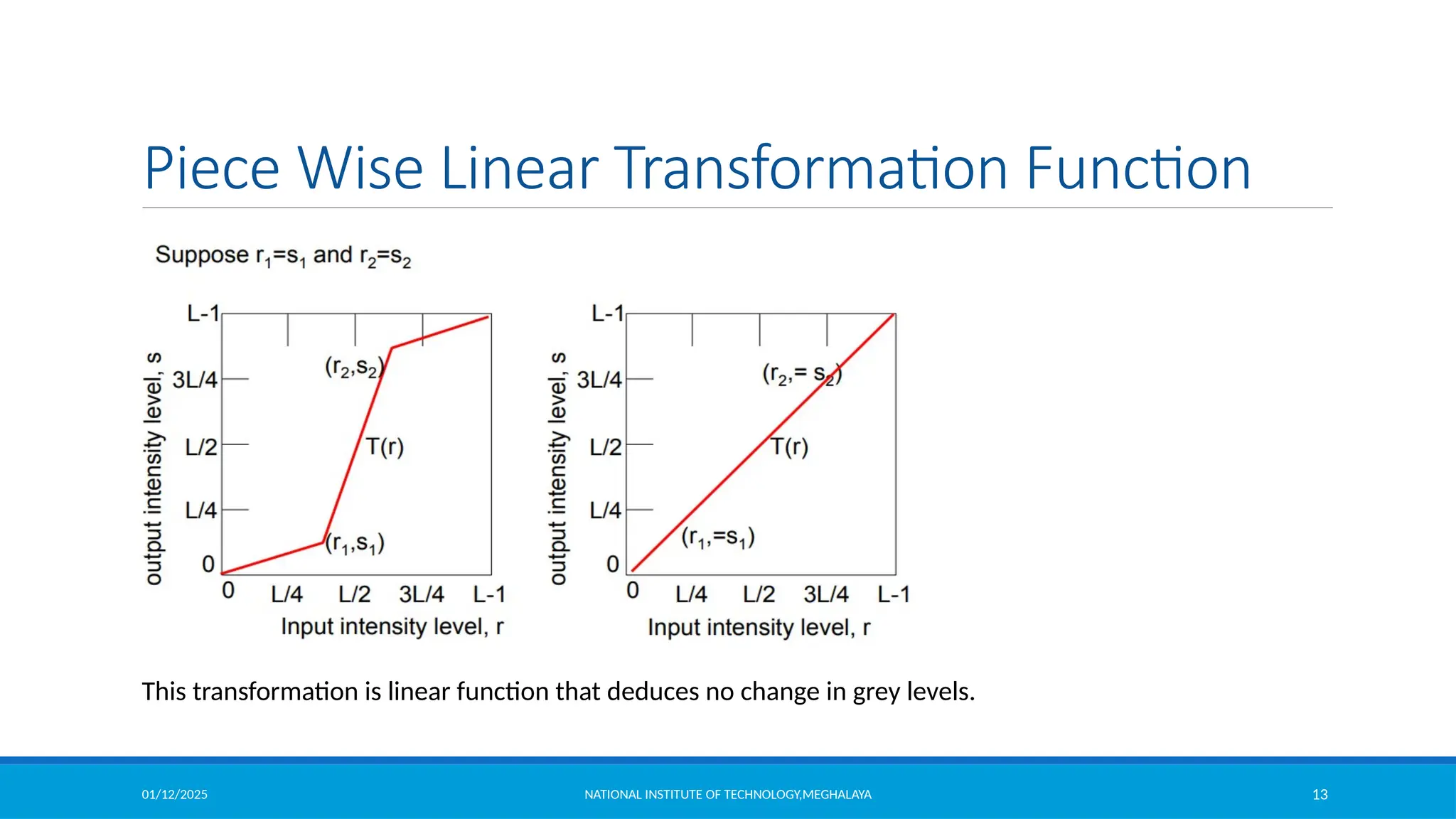
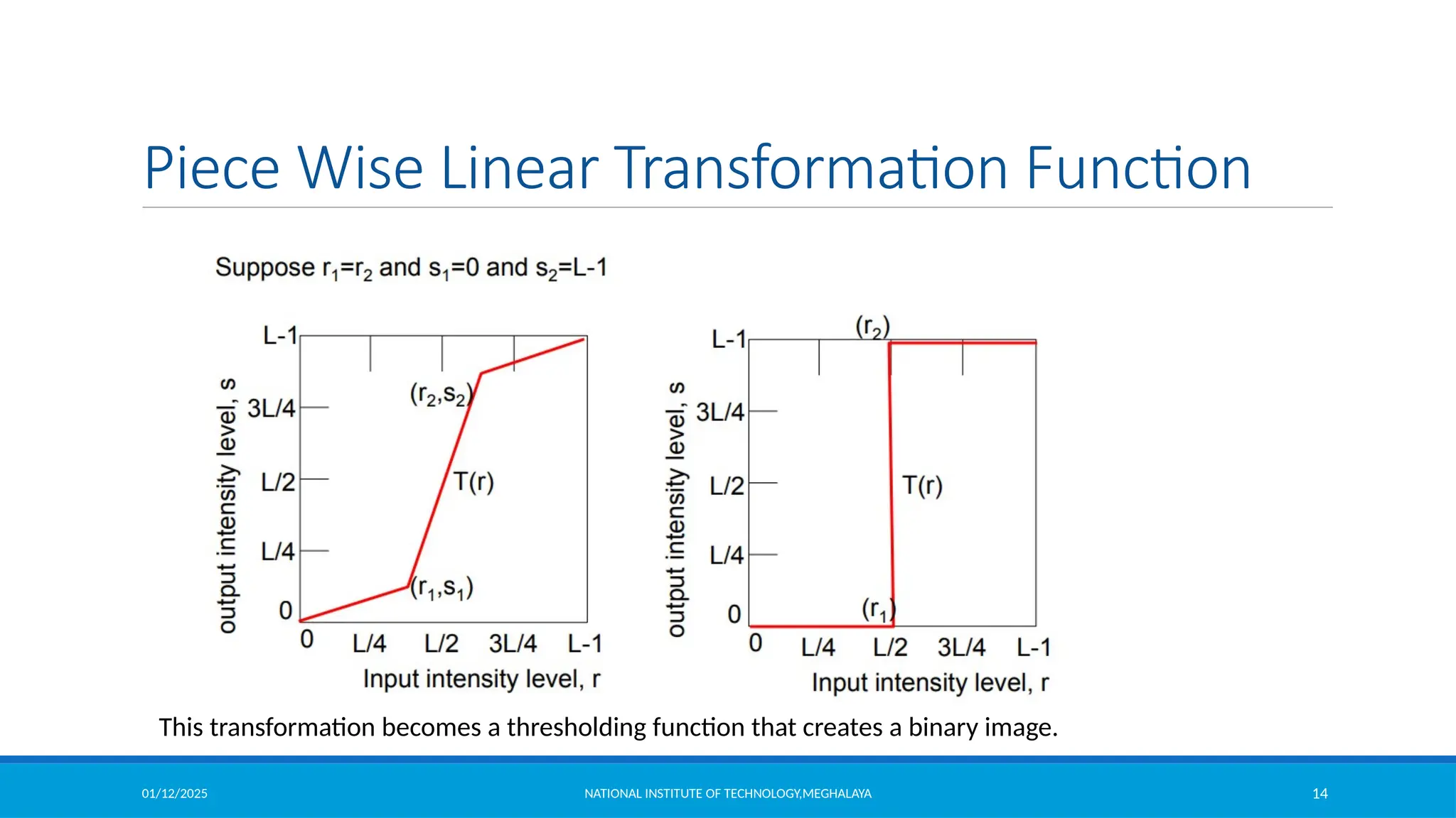
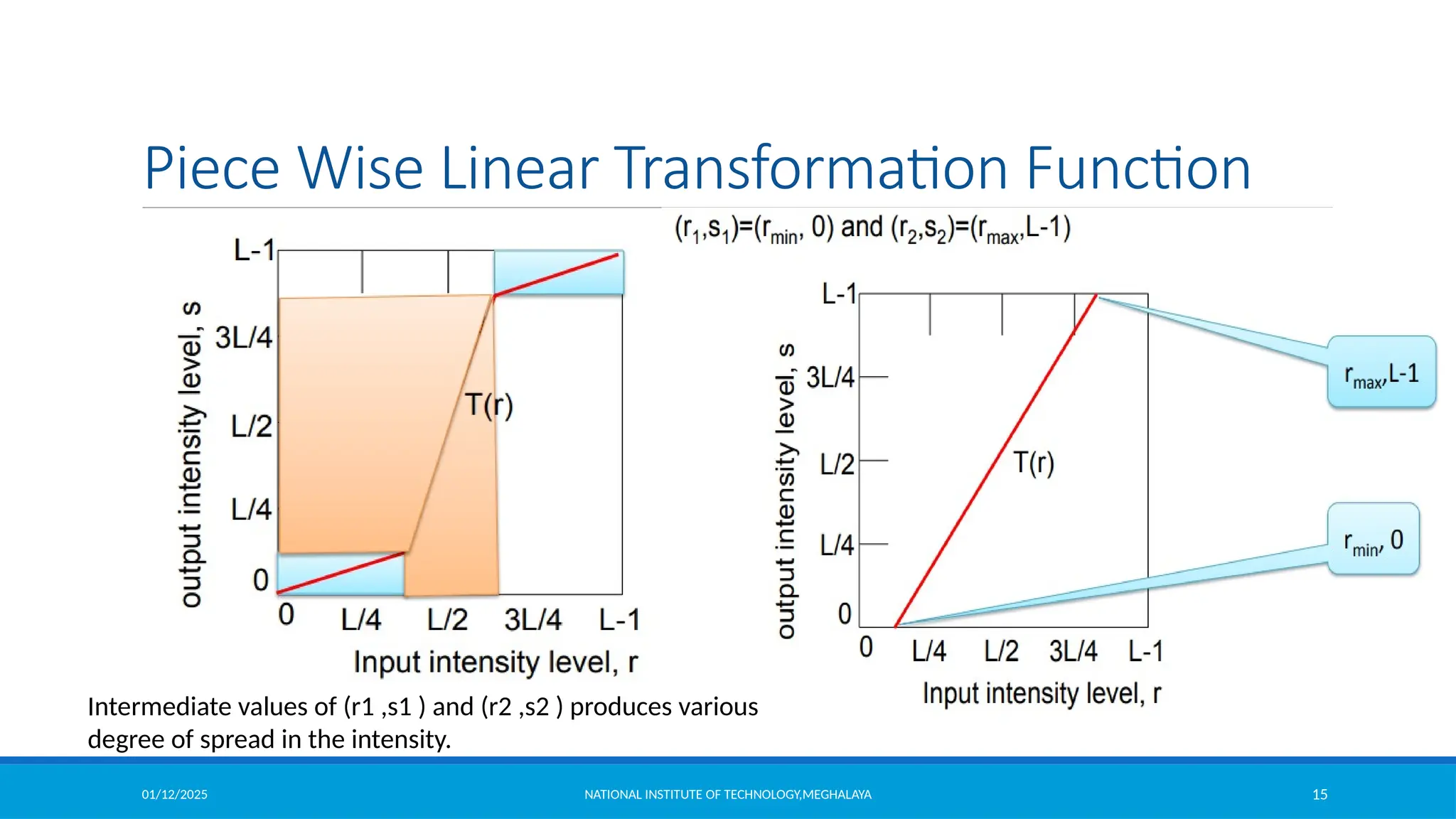
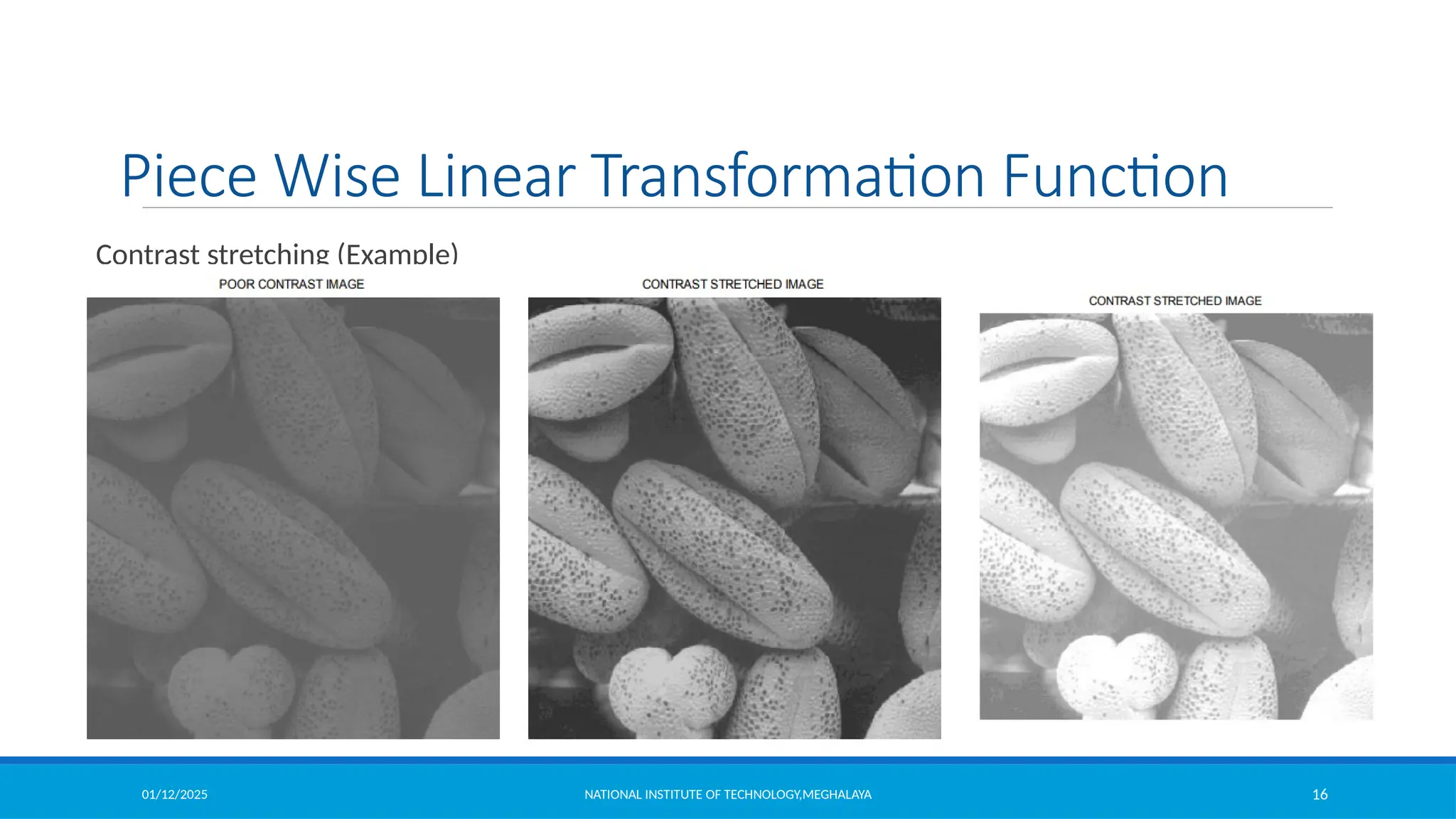
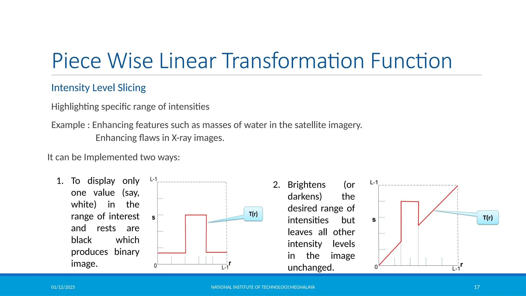
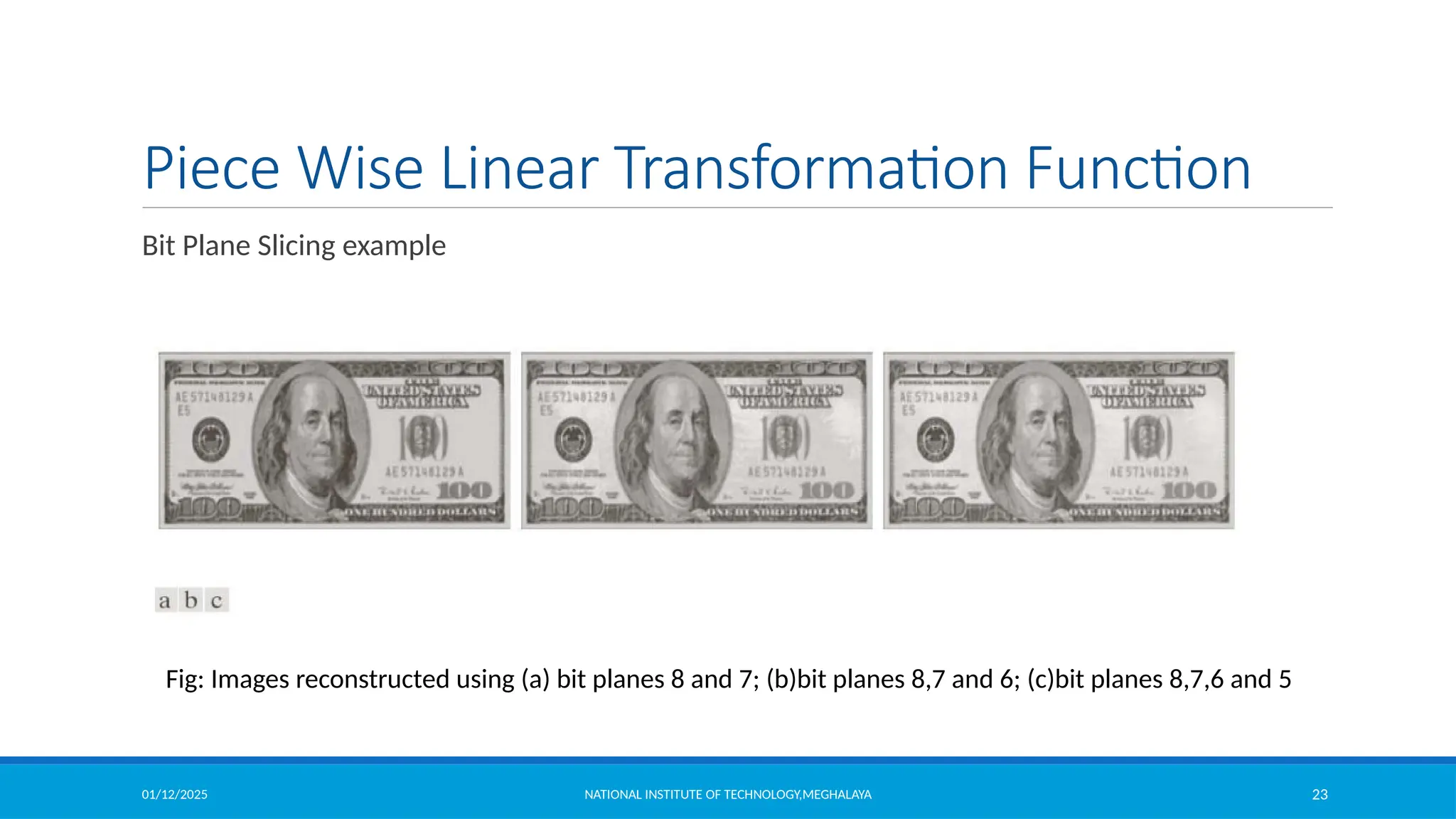
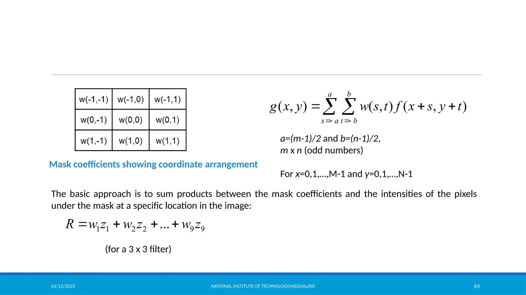
Piece Wise Linear Transformation Function
Intensity Level Slicing example
clear all;
clc;
itemp = imread('intensity_level_slicing.jpg');%read the image
image = itemp(:,:,1);
rmin = 100; %decide the min. level of intensity level slicing range
rmax = 180; %decide the max. level of intensity level slicing range
[r,c]= size(image); % get the dimensions of image
s = zeros(r,c); % pre allocate a variable to store the result image
for i = 1:r
for j = 1:c
% if the current pixel of original image is in the specfied range then make it 0 in the result image
if (rmin < image(i,j)&& image(i,j) < rmax)
s(i,j) = 0;
else
% otherwise store the same value of the pixel in the result image
s(i,j) = image(i,j);
end
end
end
figure,imshow(uint8(image)) %display original image
figure,imshow(uint8(s)) %display result image](https://image.slidesharecdn.com/module2-250112143149-8855b5c3/75/Image-Enhancement-in-Spatial-Domain-and-Frequency-Domain-19-2048.jpg)
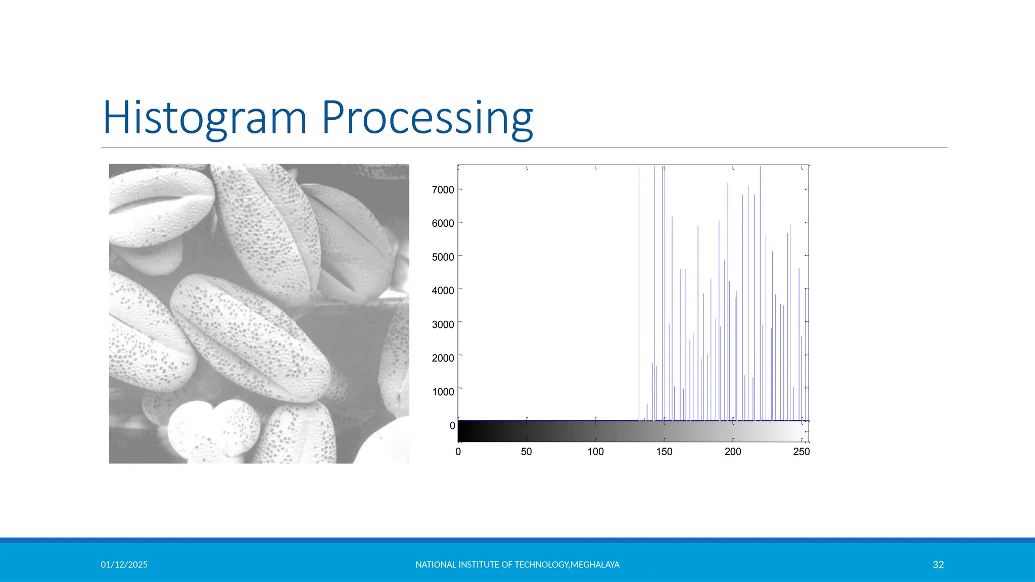
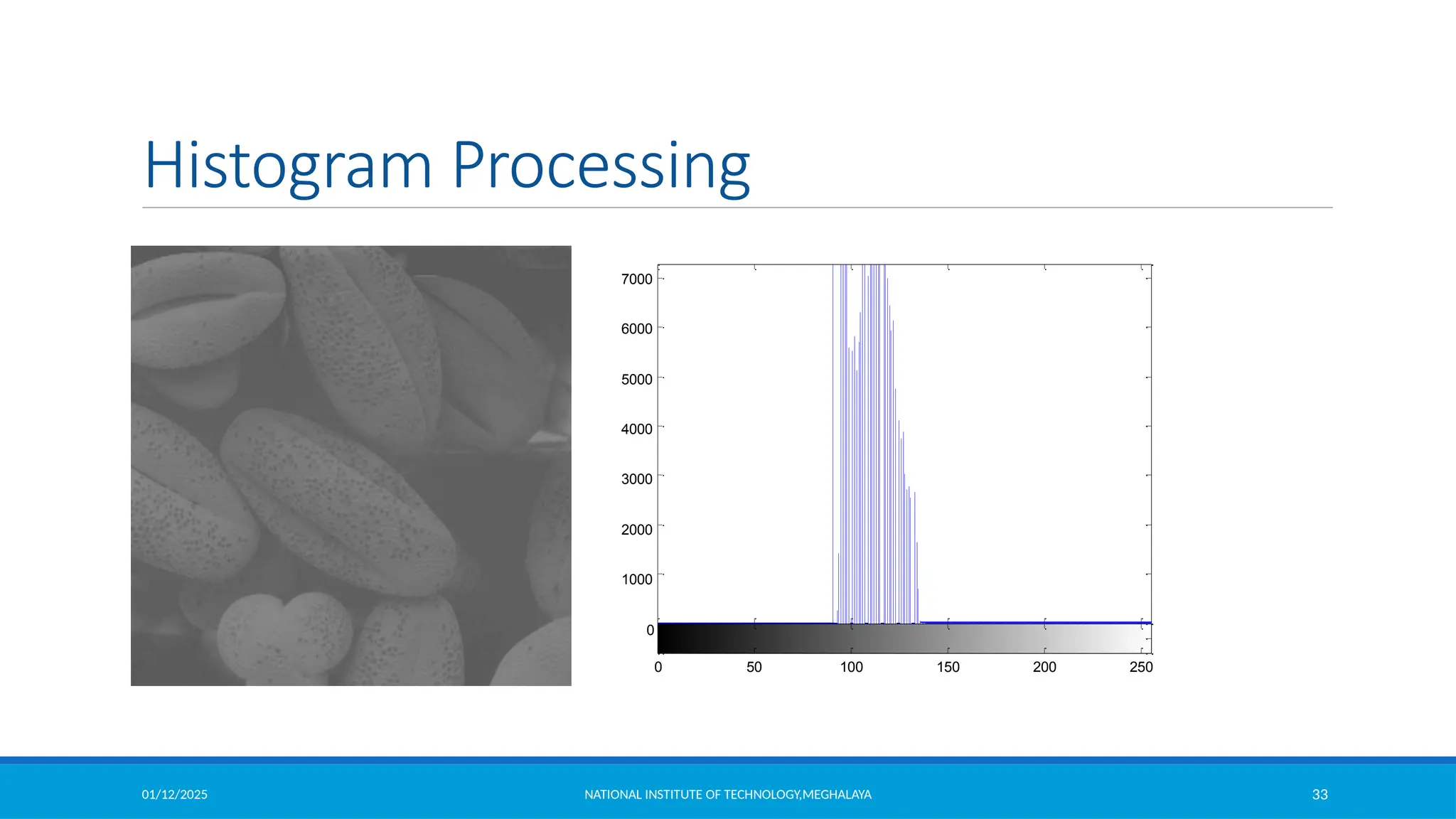
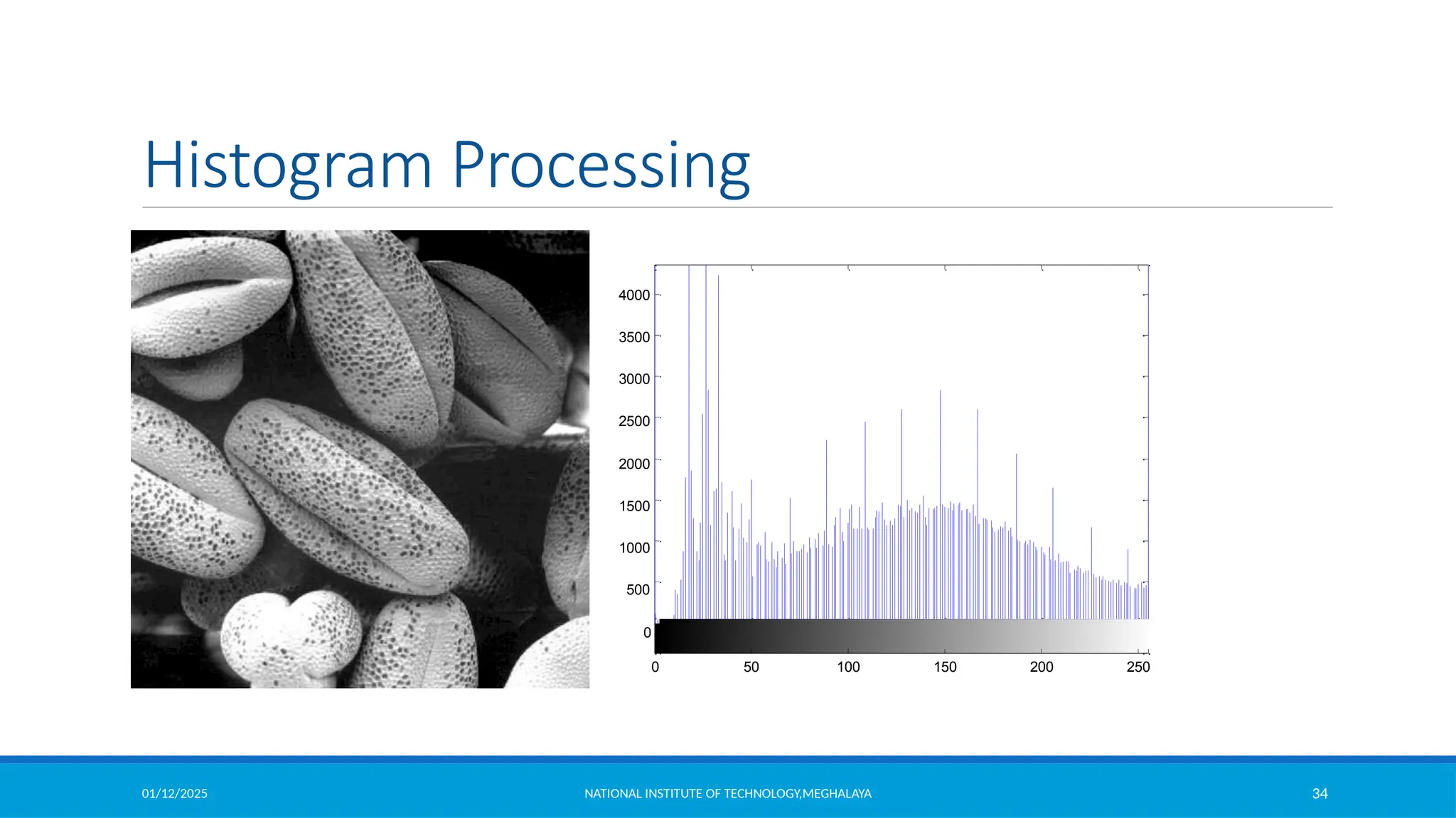
![01/12/2025 NATIONAL INSTITUTE OF TECHNOLOGY,MEGHALAYA 30
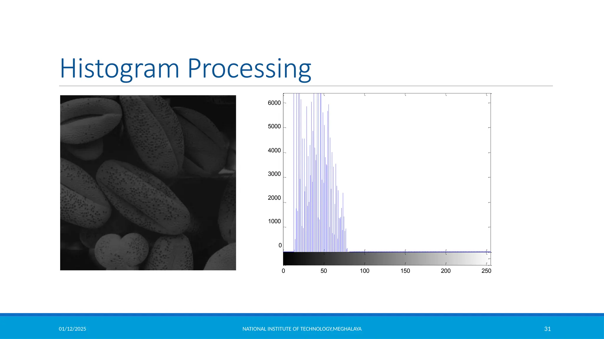
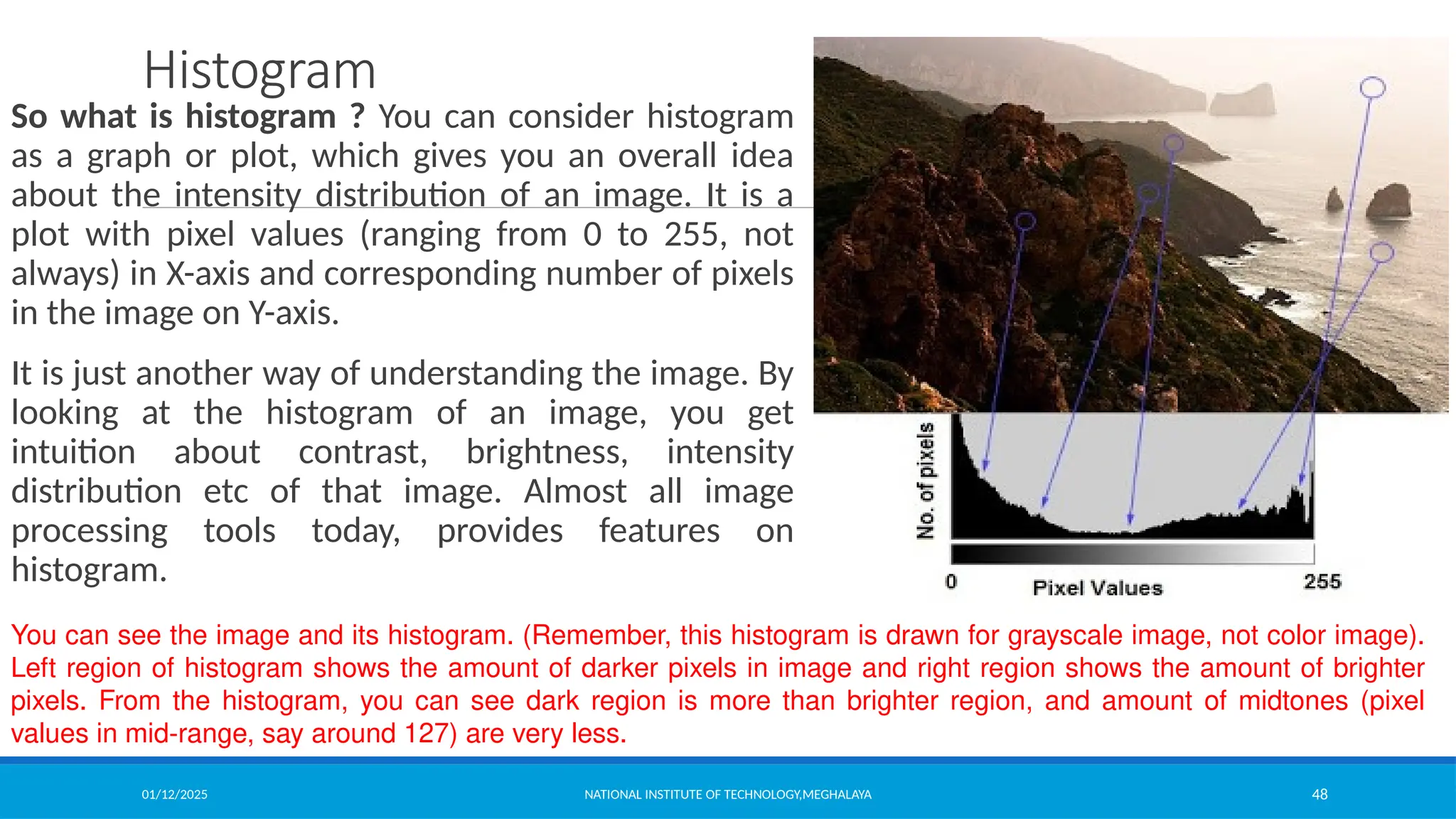
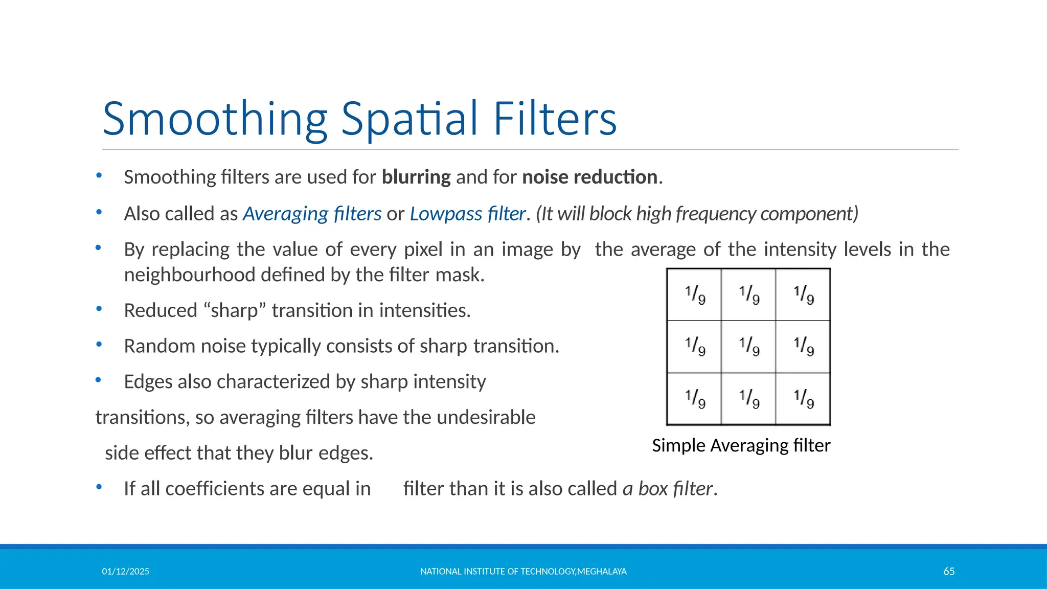
Histogram Processing
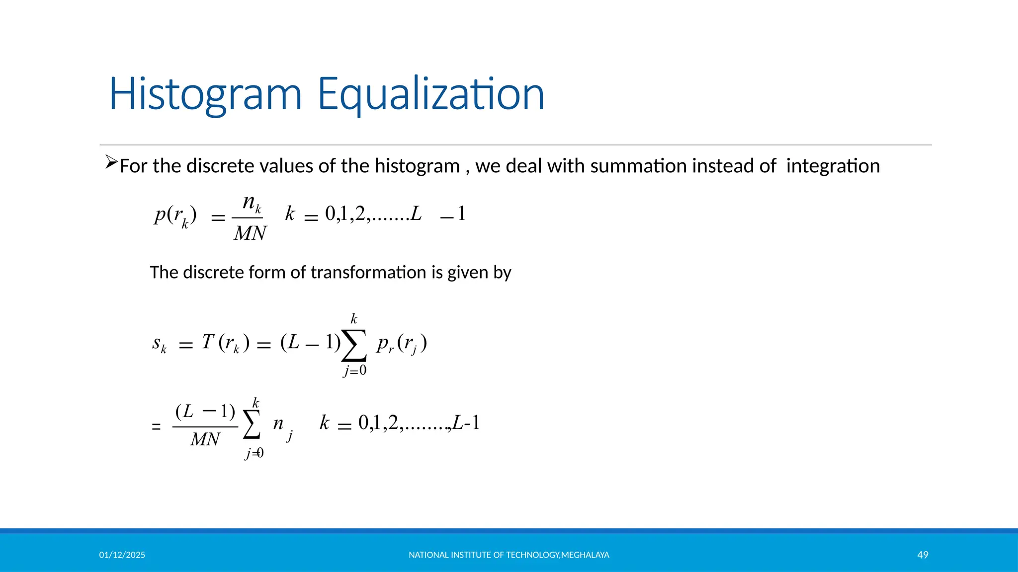
Let the intensity level in the image be in the range from [0 L-1] Histogram is a discrete function
,
where rk is the kth intensity value
nk is the number of pixels in the image with pixel level
This histogram is normalized by dividing each component by total number of pixels in the
image.
Thus normalized histogram is given by,
is an estimate of the probability of occurrence of intensity level in an image.
(Sum all the components=1)](https://image.slidesharecdn.com/module2-250112143149-8855b5c3/75/Image-Enhancement-in-Spatial-Domain-and-Frequency-Domain-30-2048.jpg)
![01/12/2025 NATIONAL INSTITUTE OF TECHNOLOGY,MEGHALAYA 40
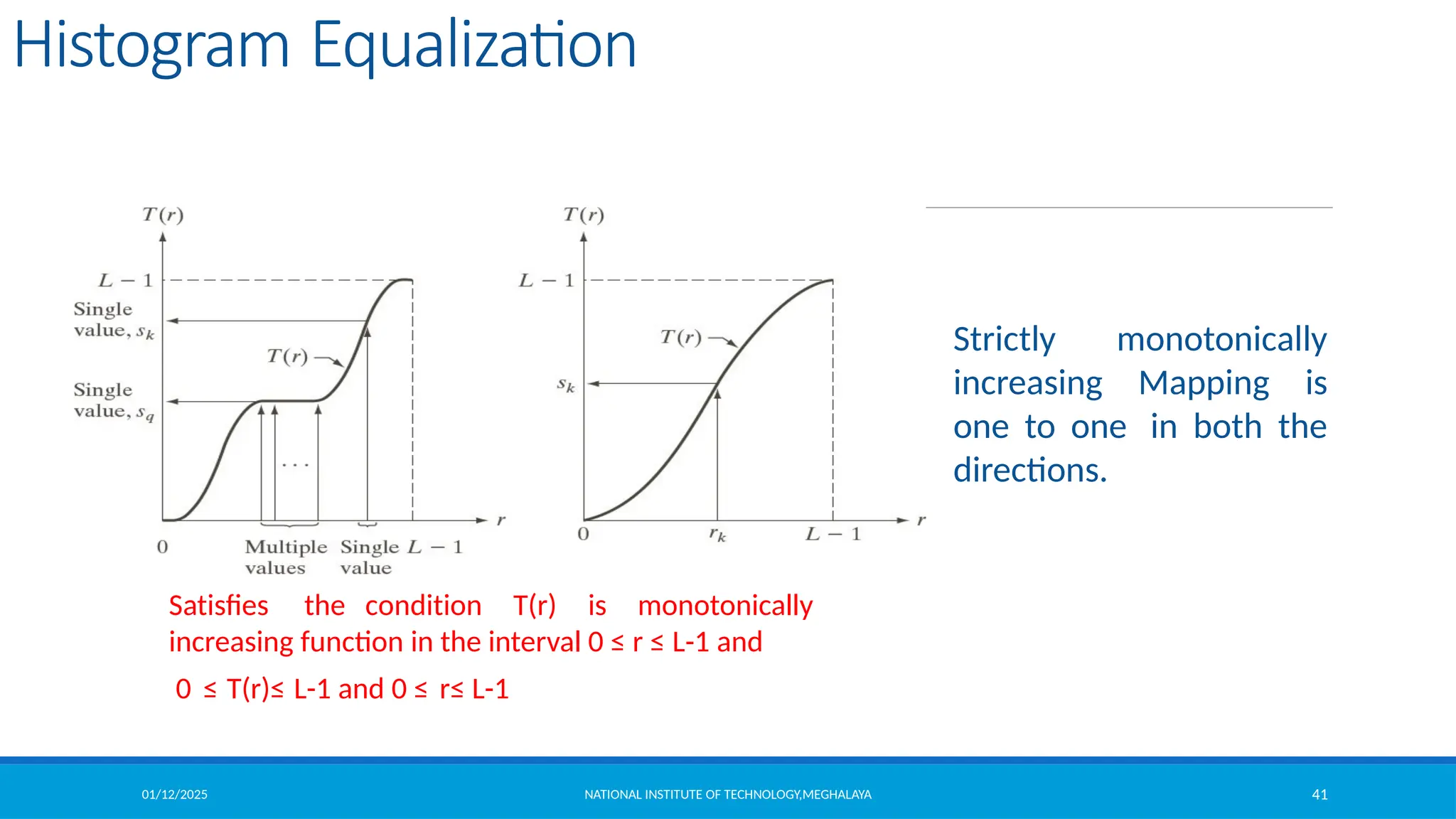
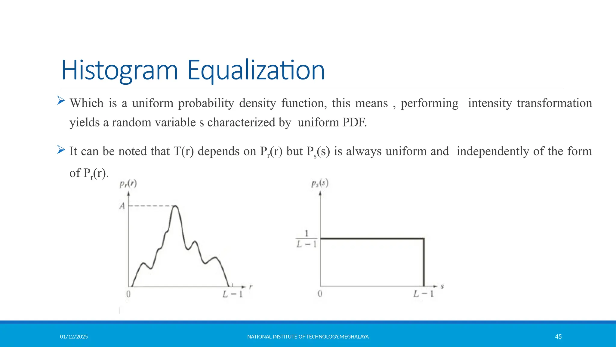
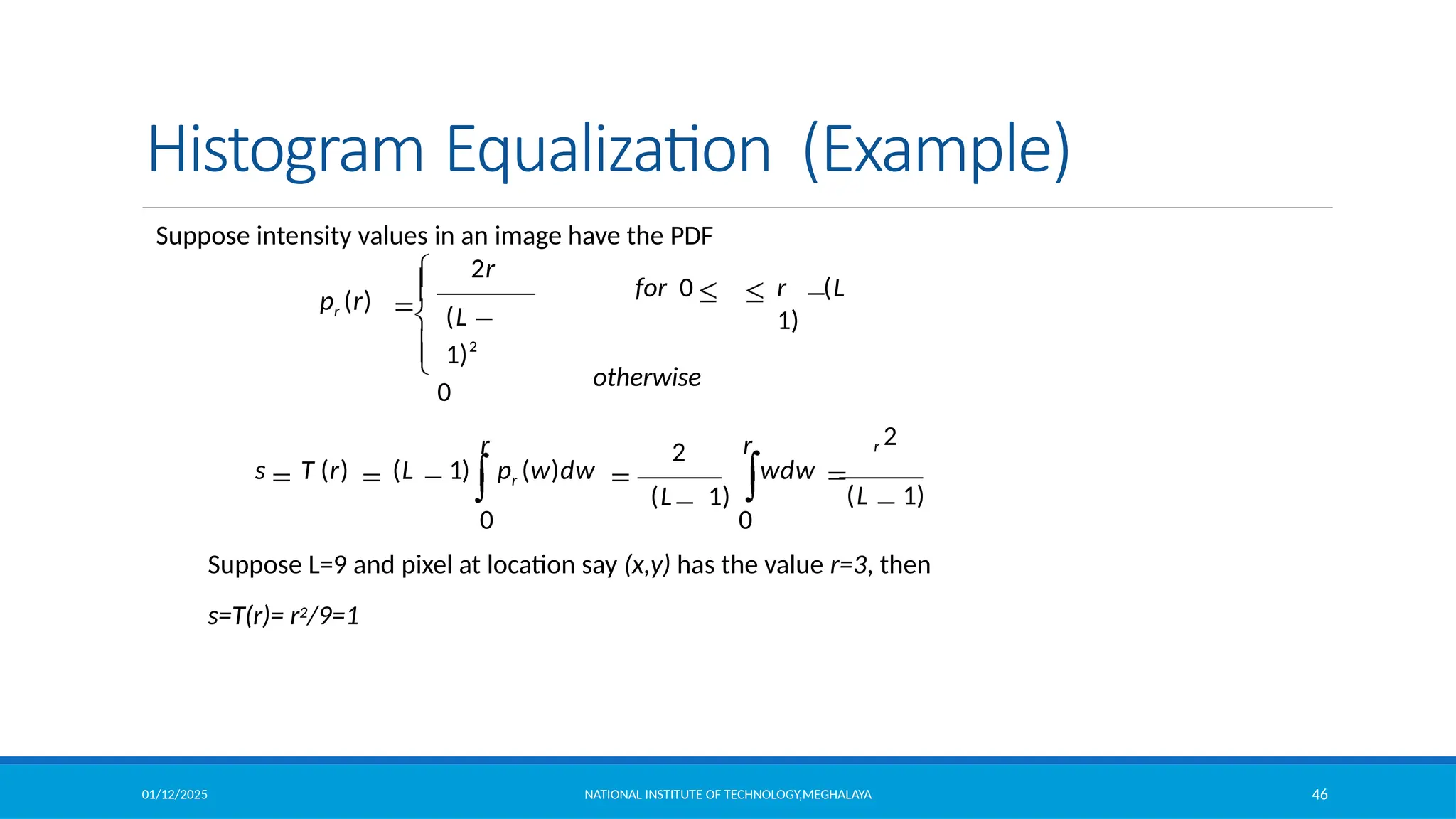
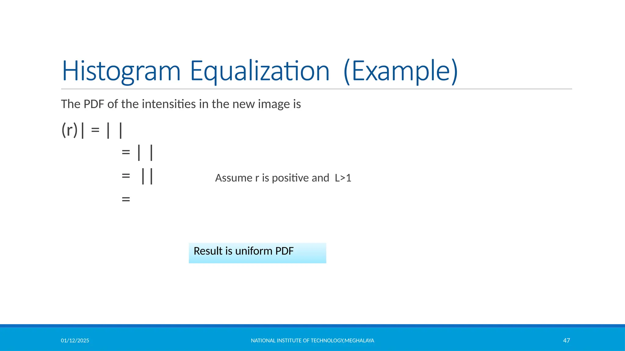
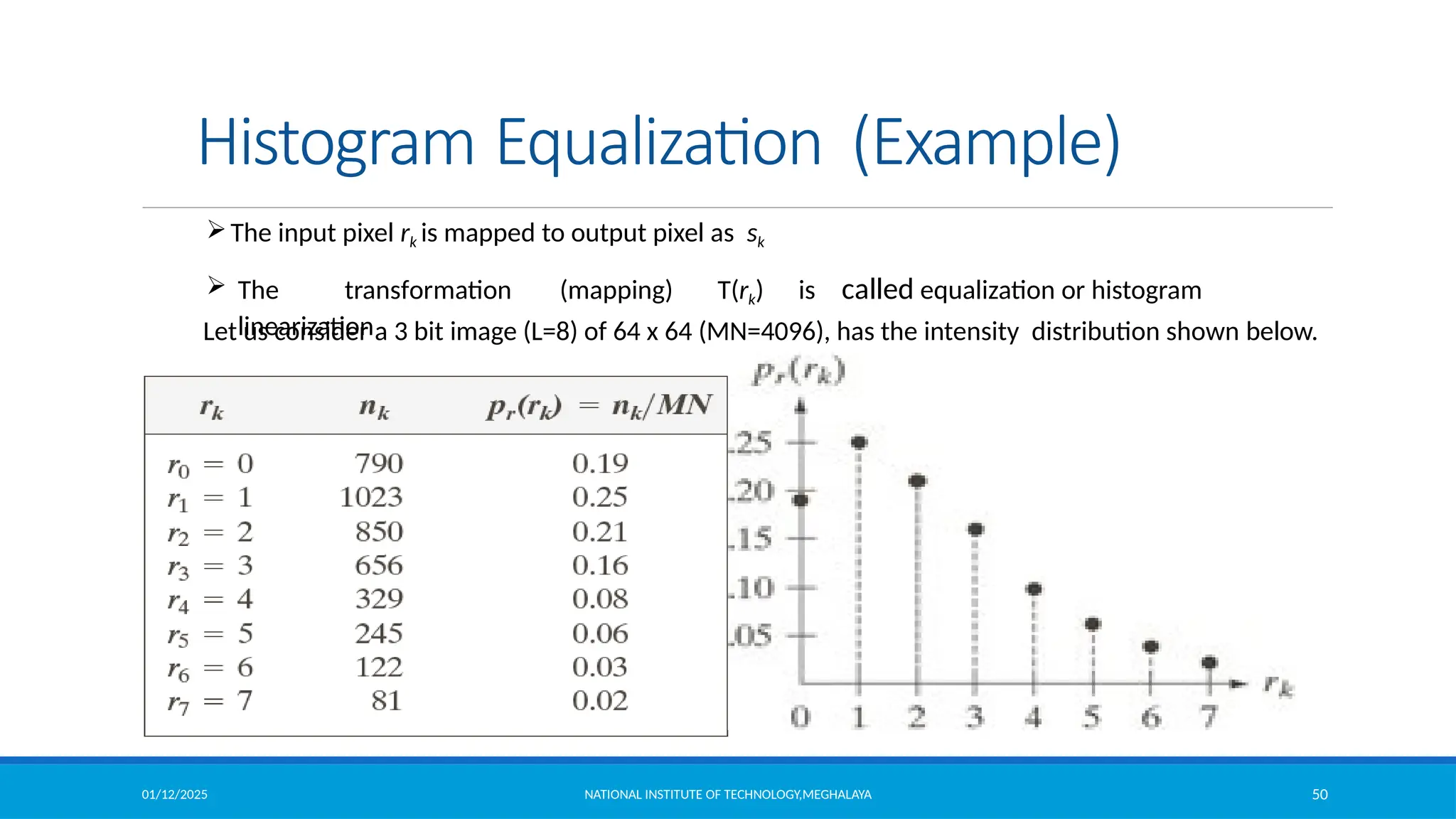
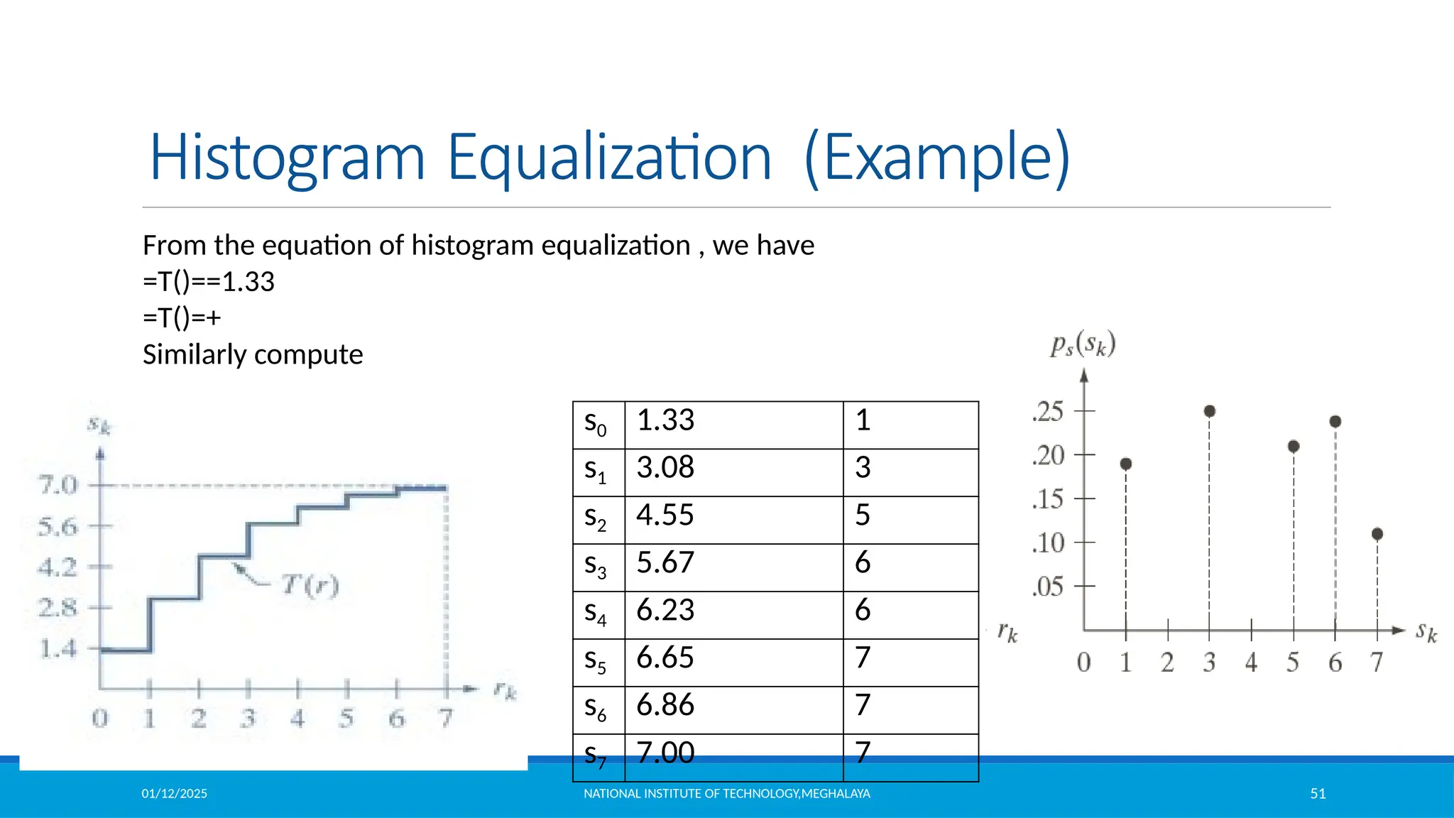
Histogram Equalization
Let us denote r [0 L-1] as intensities of the image to be processed
r=0 corresponding to black and r=L-1 representing white.
Let the intensity transformation is defined by s=T(r) , where0 ≤ r ≤ L-1
T(r) is monotonically increasing function in the interval 0 ≤ r ≤ L-1
0 ≤ T(r)≤ L-1 and 0 ≤ r ≤ L-1
Suppose we use the inverse operation as r=T-1(s) , then the condition
should be strictly monotonically increasing.](https://image.slidesharecdn.com/module2-250112143149-8855b5c3/75/Image-Enhancement-in-Spatial-Domain-and-Frequency-Domain-40-2048.jpg)
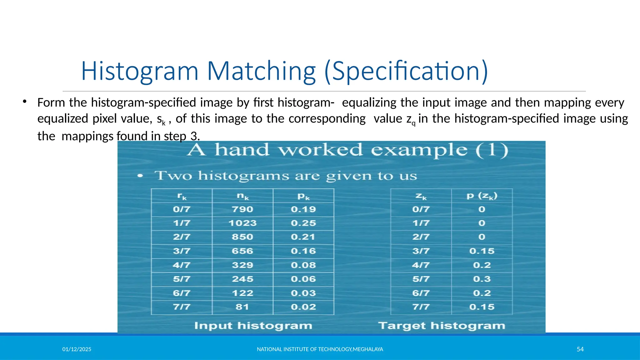
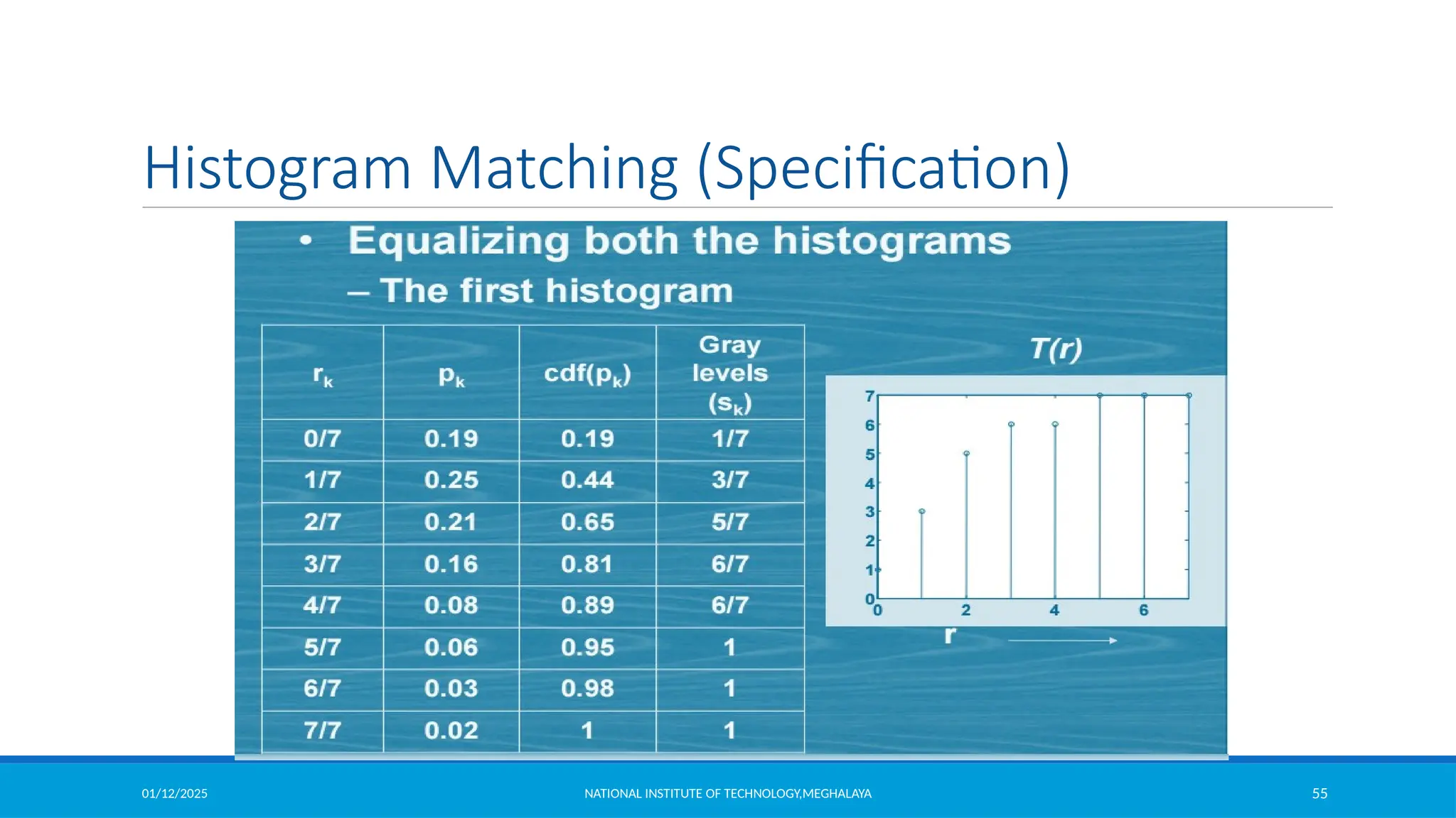
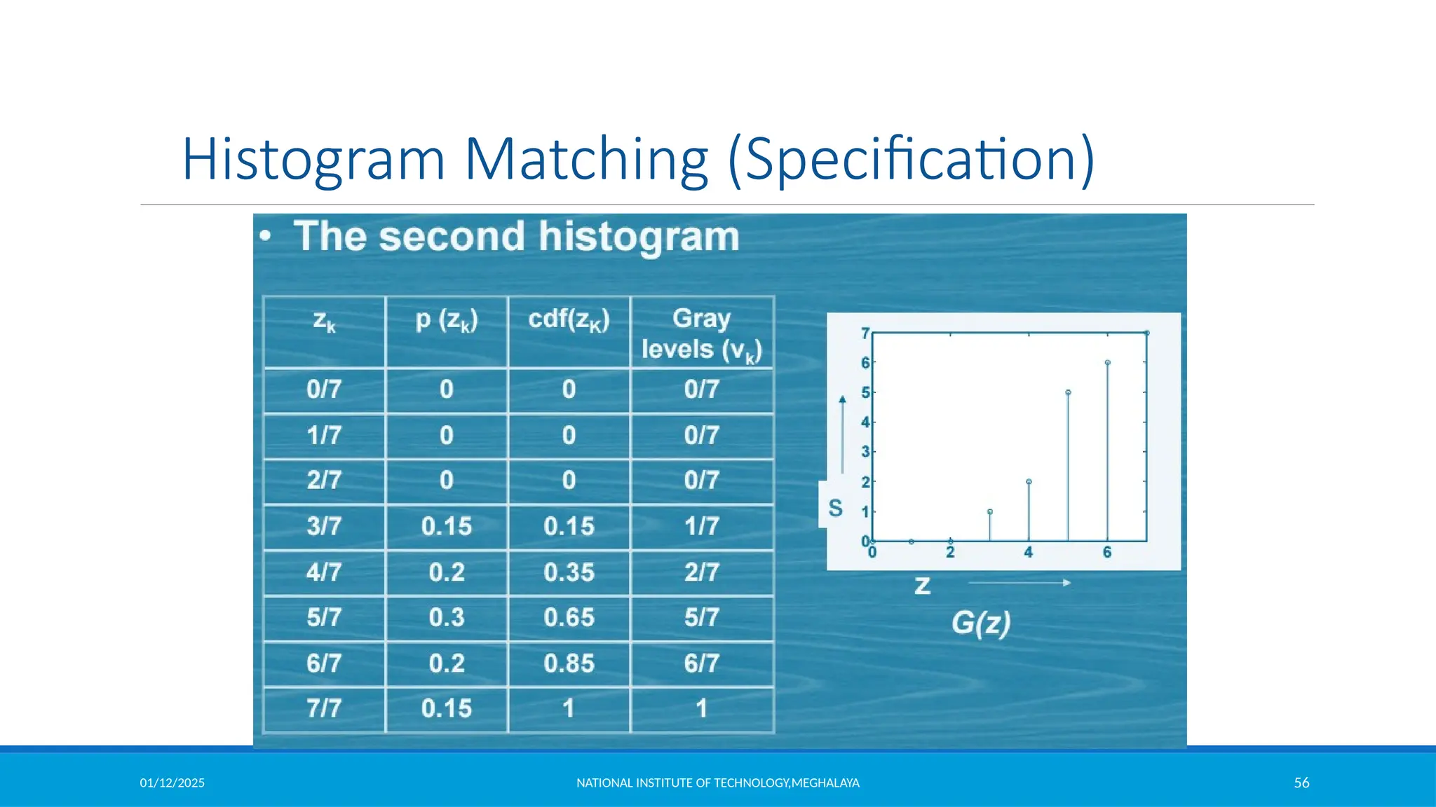
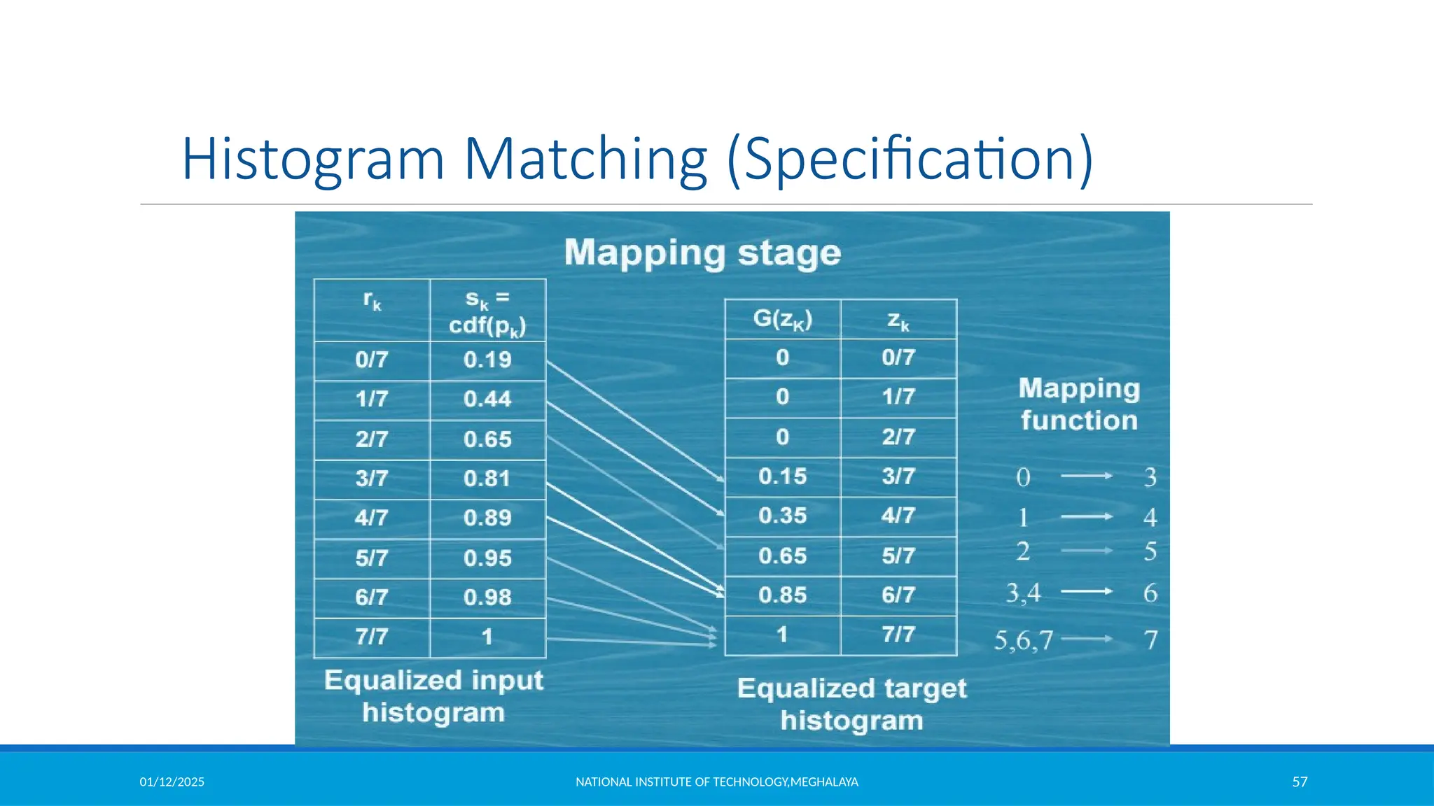
![01/12/2025 NATIONAL INSTITUTE OF TECHNOLOGY,MEGHALAYA 53
Histogram Matching (Specification)
Histogram Specification Procedure:
1. Compute the histogram pr (r) of the given image, and use it to find the histogram
equalization transformation in equation
and round the resulting values to the integer range [0, L-1]
2. Compute all values of the transformation function G using same equation G(zq ) = (L -1)
q =0,1,2,..., L -1 and round values of G
3. For every value of sk, k = 0,1,…,L-1, use the stored values of G to find the corresponding
value of zq so that G(zq) is closet to sk and store these mappings from s to z.
, k = 0,1,2,...,L -1
MN
k
j0
n j
sk = T (rk ) = (L -1)
i0](https://image.slidesharecdn.com/module2-250112143149-8855b5c3/75/Image-Enhancement-in-Spatial-Domain-and-Frequency-Domain-53-2048.jpg)
![01/12/2025 NATIONAL INSTITUTE OF TECHNOLOGY,MEGHALAYA 79
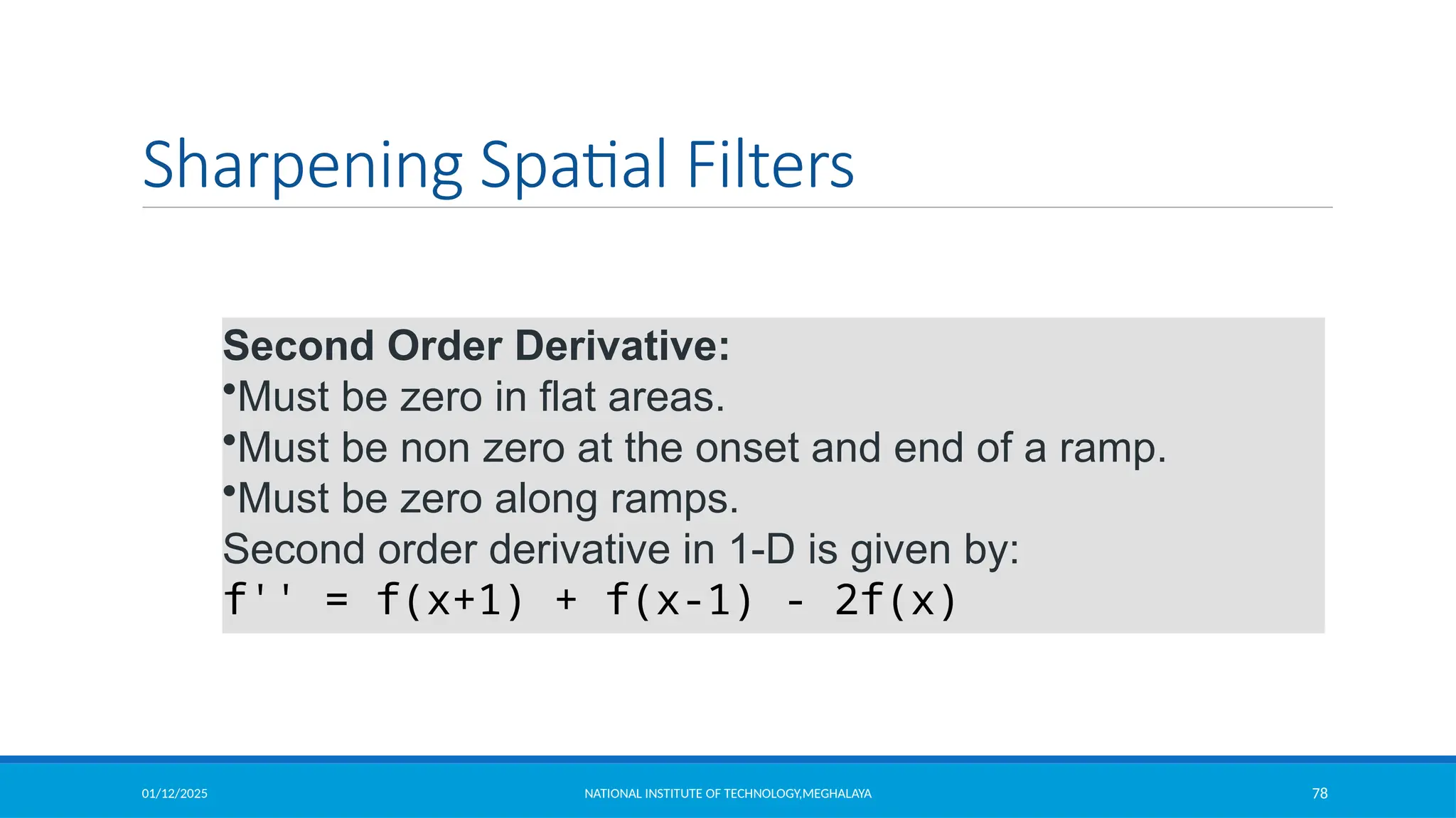
Sharpening Spatial Filters
2
2
( , 1) ( , 1) 2 ( , )
f
f x y f x y f x y
y
The first sharpening filter we will discuss is the Laplacian
– Isotropic
– One of the simplest sharpening filters
– We will look at a digital implementation
The Laplacian is defined as follows
where.,
and
2 2
2
2 2
f f
f
x y
2
2
( 1, ) ( 1, ) 2 ( , )
f
f x y f x y f x y
x
2
f [ f (x 1, y) f (x 1, y) f (x, y 1) f (x, y 1)] 4 f (x, y)](https://image.slidesharecdn.com/module2-250112143149-8855b5c3/75/Image-Enhancement-in-Spatial-Domain-and-Frequency-Domain-79-2048.jpg)
![01/12/2025 NATIONAL INSTITUTE OF TECHNOLOGY,MEGHALAYA 80
Laplacian Operator
We can easily build a filter based on 2
f. There are lots of slightly different versions of the
Laplacian that can be used:
2
f [ f (x 1, y) f (x 1,y)
f (x, y 1) f (x,1)]
4 f (x, y)
1 1 1
1 -8 1
1 1 1
We can easily build a filter based on 2
f. There are lots of slightly different versions of the
Laplacian that can be used:
-1 -1 -1
-1 8 -1
-1 -1 -1
0 1 0
1 -4 1
0 1 0
0 1 0
1 -4 1
0 1 0
2
f [ f (x 1, y) f (x 1,y) f (x, y
1) f (x,y1)+ f (x 1, y+1) f (x +1,y-
1) f (x+1, y 1) f (x+1,y1] 8 f (x, y](https://image.slidesharecdn.com/module2-250112143149-8855b5c3/75/Image-Enhancement-in-Spatial-Domain-and-Frequency-Domain-80-2048.jpg)

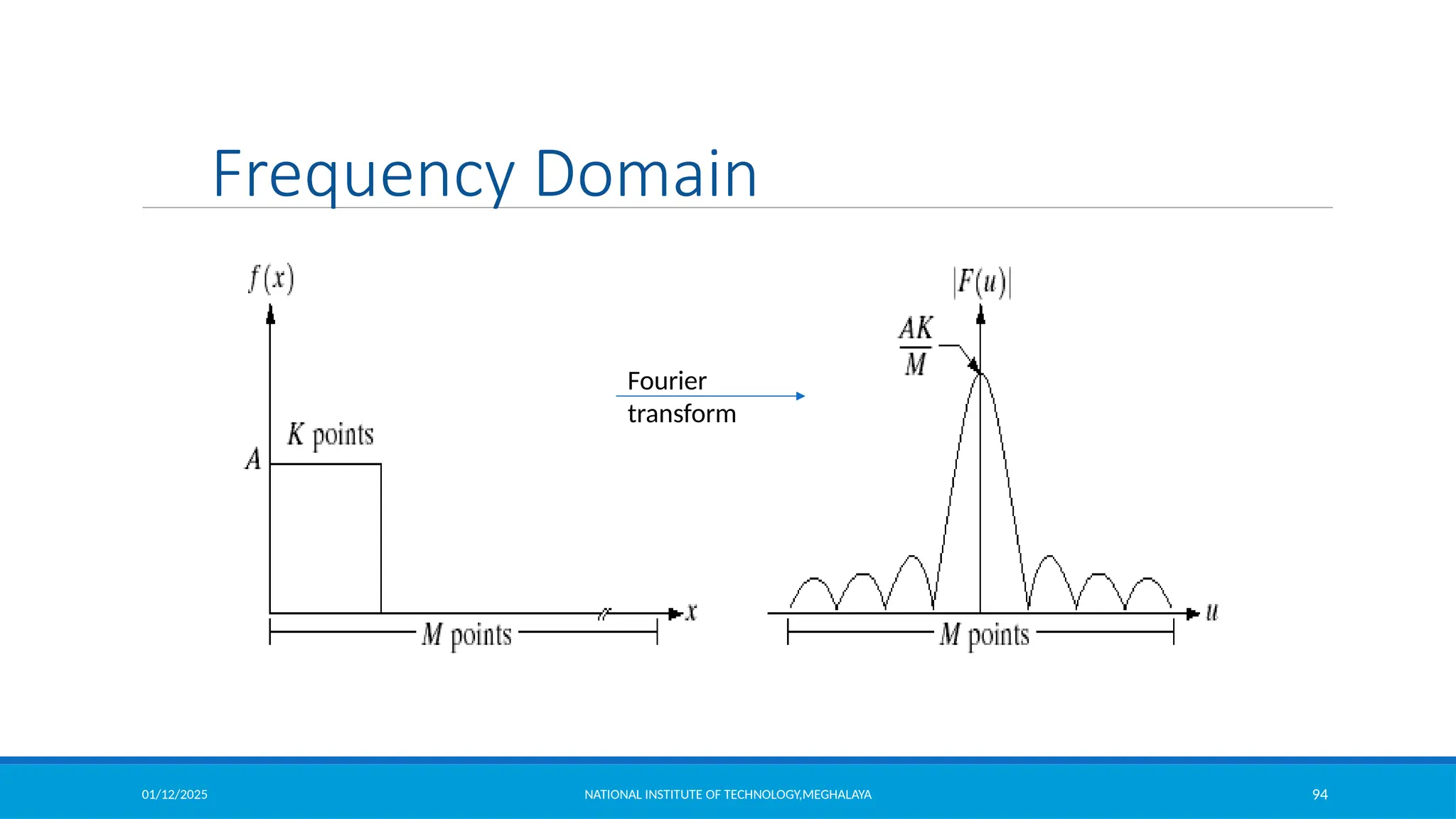
![01/12/2025 NATIONAL INSTITUTE OF TECHNOLOGY,MEGHALAYA 93
Frequency Domain
frequency domain
sin
cos j
e j
j
1
cos
sin
]
2
sin
2
)[cos
(
1
)
(
1
0
x
M
u
j
x
M
u
x
f
M
u
F
M
x
Euler’s formula:
frequency
u
F(u)
for x = 0, 1, 2…M-1 and y = 0, 1, 2…N-1](https://image.slidesharecdn.com/module2-250112143149-8855b5c3/75/Image-Enhancement-in-Spatial-Domain-and-Frequency-Domain-93-2048.jpg)
![01/12/2025 NATIONAL INSTITUTE OF TECHNOLOGY,MEGHALAYA 95
Complex Quantities to Real Quantities
Useful representation
2
/
1
2
2
)]
,
(
)
,
(
[
)
,
( v
u
I
v
u
R
v
u
F
]
)
,
(
)
,
(
[
tan
)
,
( 1
v
u
R
v
u
I
v
u
magnitude
phase
)
,
(
)
,
(
)
,
(
)
,
( 2
2
2
v
u
I
v
u
R
v
u
F
v
u
P
Power spectrum](https://image.slidesharecdn.com/module2-250112143149-8855b5c3/75/Image-Enhancement-in-Spatial-Domain-and-Frequency-Domain-95-2048.jpg)