description of line attributes in computer graphics

1. BY
Ms. N. RUBA.,MCA.,M.Phil.,(Ph.D).,
Assistant Professor of CA,
Bon Securs College for Women,
Thanjavur.
COMPUTER GRAPHICS
Attributes of output primitives

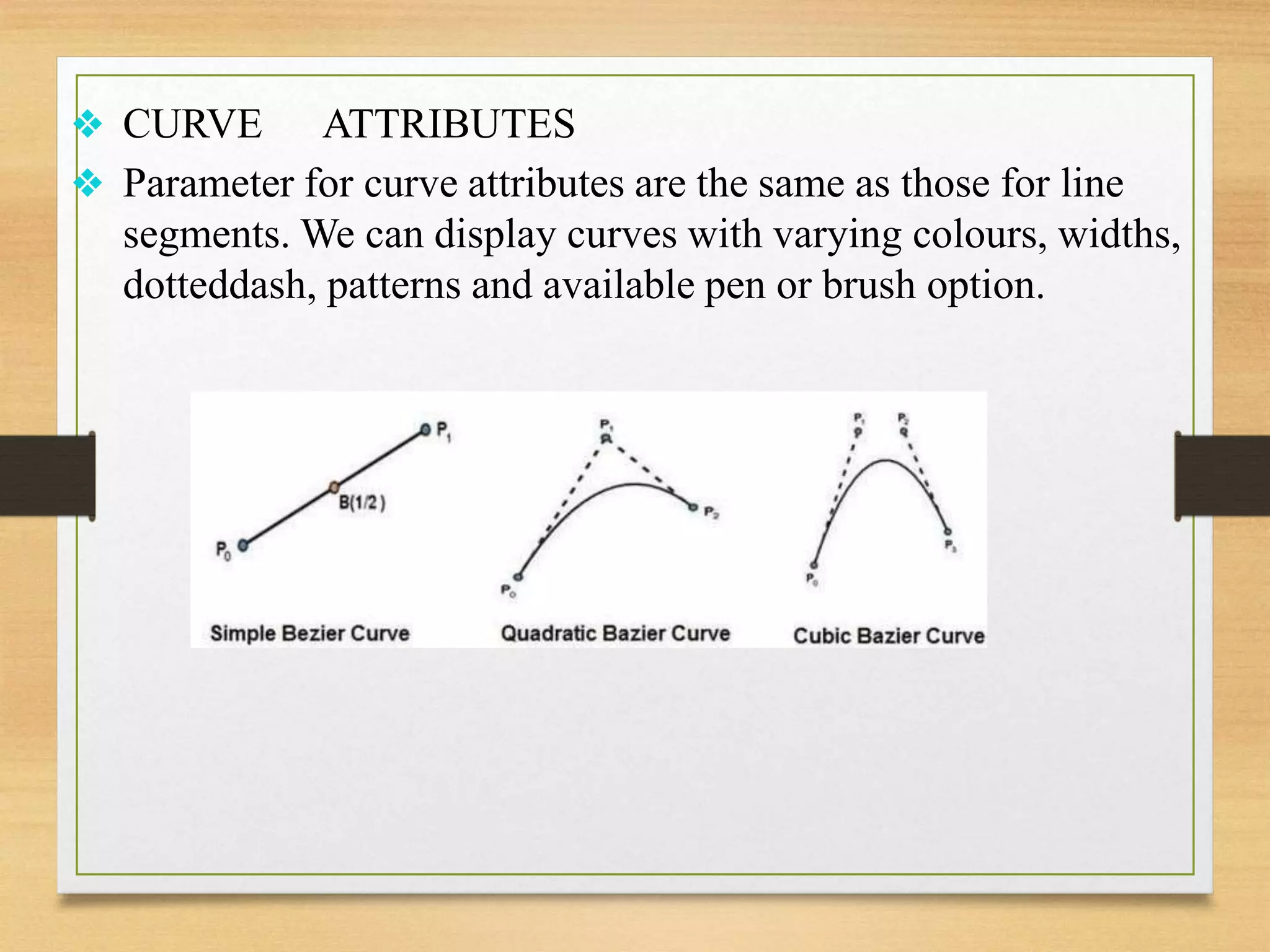
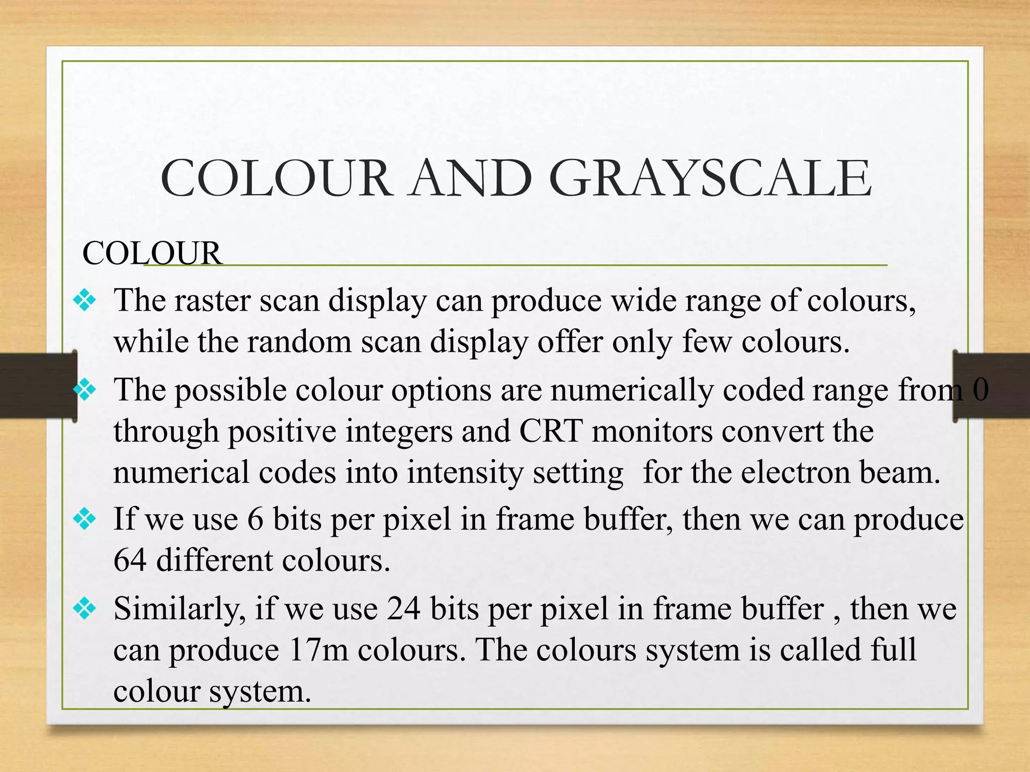
2. Attributes of output primitives
❖ Any parameter that affects the way a primitive is to be
displayed id referred to as an attribute parameter.
❖ It is used to determine the fundamental characteristics of a
primitive.
❖ There are various types of attributes. In this presentation we
are going to learn about three attributes.the attributes are,
❖ Line attribute
❖ Curve attribute
❖ Colour and Gray scale level

3. Attributes
LINE ATTRIBUTES
✔ Basic attributes of a straight line segment are its type
,its width, and its colour.
LINE TYPE
▪ Solid lines
▪ Dashed lines
▪ Dotted lines
▪ Dashed dotted lines
❖ A dashed line could be displayed by generating an
inter dash spacing that is equal to the length of the
solid section. Both the length of the dashes and the
inter dash spacing are often specified as user option.

4. Attributes
.
❖A dotted line can be displayed by generating
very short dashes with the spacing equal to or
greater than the dash size. Similar methods are
used to produce other line-type variation.
❖To set line-type attributes in a graphics
application program, a user invokes the
function,
Set Line-type(It)
❖Where parameter It is assigned a positive integer
value of 1,2,3 or 4 to generate lines that are
respectively solid, dashed, dotted or dash-dotted.

5. LINE WIDTH
❖ Line-width parameter 1r is assigned a positive number
to indicate the relative width of the line to be
displayed. A value of 1 specifies a standard-width line
on.
❖ For line with slope magnitude greater than 1, we can
plot thick lines with horizontal spans, alternately
picking up pixels to the right and left of the line path.
❖ Problems with implementing width options using
horizontal or vertical pixel spans is that the method
produces lines whose ends are horizontal or vertical
regardless of the slope of the line.

6. LINE WIDTH
❖ Problems with implementing width options using
horizontal or vertical pixel spans is that the method
produces lines whose ends are horizontal or vertical
regardless of the slope of the line.
❖ This effect is more noticeable with very thick lines. We
can adjust the shape of the lines ends to give them a
better appearance by adding line caps.
❖ One kind of line cap is the butt cap obtained by
adjusting the end positions of the component parallel
lines so that the thick line is displayed with square ends
that are perpendicular to the line path. If the specified
line has slope m, the square end of the thick line has
slope
-1/m.

7. ❖Another line cap is the round cap obtained by
adding a filled semicircle to each butt cap. The
circular arcs are center on the line end-points and
have a diameter equal to the line thickness.
❖A third type of the line cap is the projecting
square cap. Here, we simply extend the line and
add butt cap that are positioned one-half of the
line width beyond the specified endpoints.
❖We can generate thick poly lines that are smoothly
joined at the cost of additional processing at the
segment end points.

8. ❖ Can generate thick poly lines that are smoothly joined at
the cost of additional processing at the segment end
points.
❖ A miter join is accomplished by extending the outer
boundaries of each of the two lines until they meet.
❖ A rounded join is produced by capping the connection
between the two segments with a circular boundary
whose diameter is equal to the line width.
❖ And a bevel join is generated by displaying the line
segments with butt caps and filling in the triangular gap
where the segments meet.

9. PEN AND BRUSH OPTION
❖ Lines can be displayed with pen or brush selections.
Options in this category include shape, size and pattern.
❖ These shapes can be stored in a pixel mask that identifies
the array of pixels positioning that are to be set along the
line path.
❖ Lines generated with pen or brush shapes can be displayed
in various widths by changing the size of the mask.

10. LINE COLOR
❖ When a system provides colour or intensity option, a
parameter giving the current.
❖ Colour index is included in the list of system attribute
values. A poly line Routine displays a line in the current
colour by setting this colour value in the frame buffer at
pixel locations along the line path using the set pixel
procedure.
❖ The number of colour choices depends on the number of
bits available per pixel in the frame buffer. We set the
line colour value in graphics with the function,
Set poly line colour
index (Ie)

11. ❖ CURVE ATTRIBUTES
❖ Parameter for curve attributes are the same as those for line
segments. We can display curves with varying colours, widths,
dotteddash, patterns and available pen or brush option.

12. COLOUR AND GRAYSCALE
COLOUR
❖ The raster scan display can produce wide range of colours,
while the random scan display offer only few colours.
❖ The possible colour options are numerically coded range from 0
through positive integers and CRT monitors convert the
numerical codes into intensity setting for the electron beam.
❖ If we use 6 bits per pixel in frame buffer, then we can produce
64 different colours.
❖ Similarly, if we use 24 bits per pixel in frame buffer , then we
can produce 17m colours. The colours system is called full
colour system.

13. GRAYSCALE
❖ In black and white monitors, colour functions can be used in
programs to set the shades of gray or gray scale.
❖ Numeric values from 0 to 1 can be used to specify the gray
scale levels which are then converted into binary codes.

14. COLOUR AND GRAYSCALE
COLOUR
❖ The raster scan display can produce wide range of colours,
while the random scan display offer only few colours.
❖ The possible colour options are numerically coded range from 0
through positive integers and CRT monitors convert the
numerical codes into intensity setting for the electron beam.
❖ If we use 6 bits per pixel in frame buffer, then we can produce
64 different colours.
❖ Similarly, if we use 24 bits per pixel in frame buffer , then we
can produce 17m colours. The colours system is called full
colour system.

15. Thank you