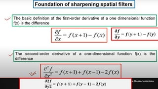
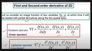
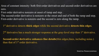
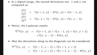
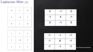
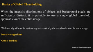
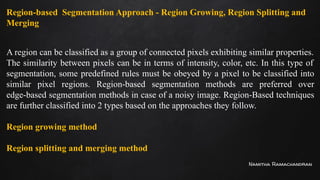
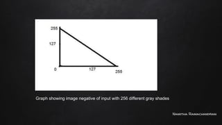
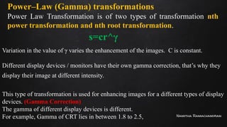
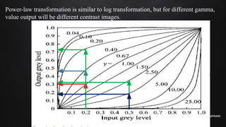
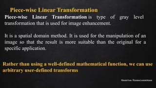
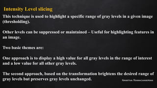
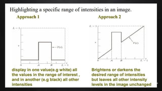
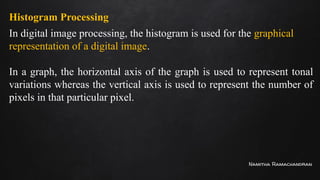
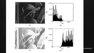
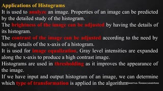
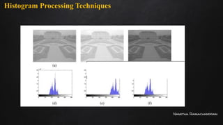
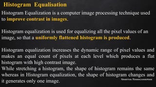
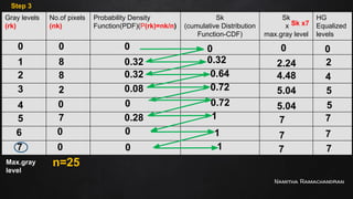
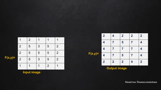
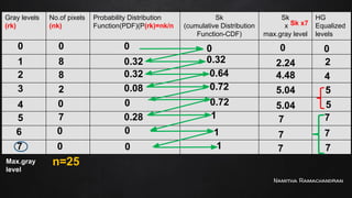
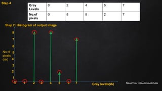
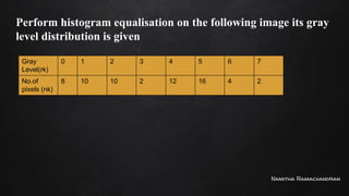
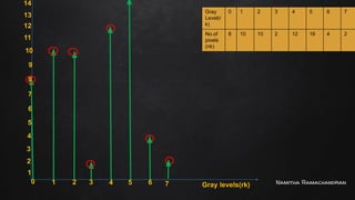
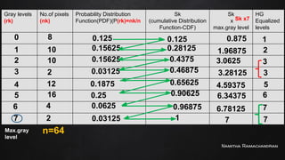
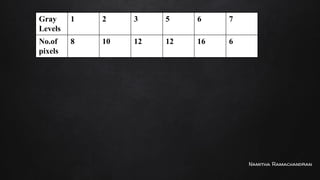
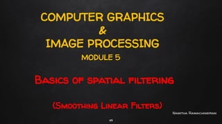
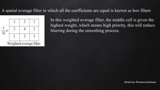
The document covers image enhancement techniques in computer graphics, specifically focusing on gray level transformations, including linear, logarithmic, and power-law transformations. It also discusses methods for contrast stretching, histogram equalization, and spatial filtering, emphasizing the importance of enhancing image quality for better visual representation. Additionally, it details the process of histogram equalization, including step-by-step calculations of frequency and probability distributions of gray levels.


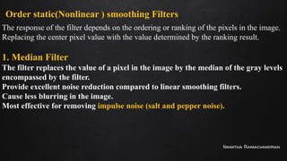
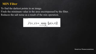
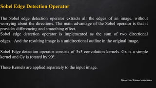
![Namitha Ramachandran
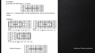
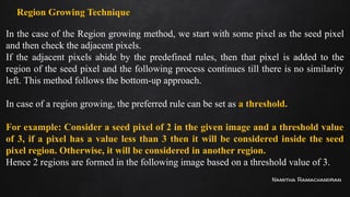
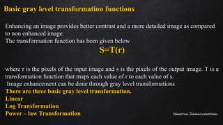
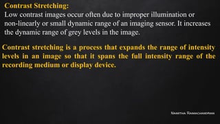
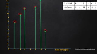
20 30 50 80 100
30 20 80 100 100
20 30 60 10 110
40 30 70 40 100
50 60 80 30 90
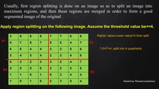
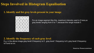
Apply standard average filter for pixel at (3,3)
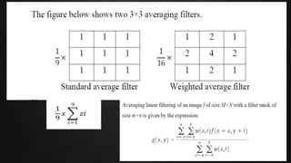
1 1 1
1 1 1
1 1 1
1/9 [20x1+80x1+100x1+30x1+60x1+10x1+30x1+70x1+40x1]
Pixel at (3,3) is 60](https://image.slidesharecdn.com/cg-5-250121101151-98d665d8/85/Computer-graphics-is-drawing-pictures-by-using-computer-aided-methods-and-algorithms-58-320.jpg)
![Namitha Ramachandran
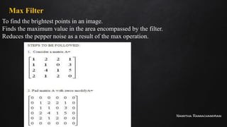
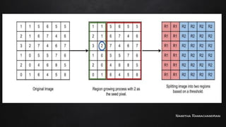
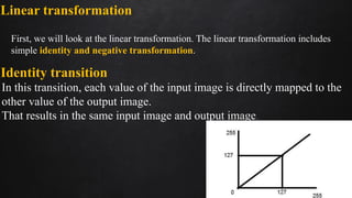
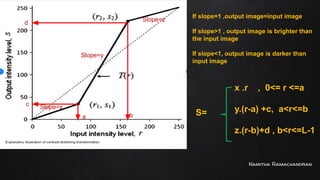
20 30 50 80 100
30 20 80 100 100
20 30 60 10 110
40 30 70 40 100
50 60 80 30 90
Apply standard average filter for pixel at (1,1)
1/9 [0x1+0x1+0x1+0x1+20x1+30x1+0x1+30x1+20x1]
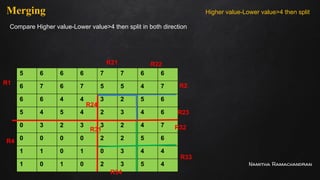
Pixel at (1,1) is 20
0
0
0
0
0
0 0 0 0 0 0
1 1 1
1 1 1
1 1 1](https://image.slidesharecdn.com/cg-5-250121101151-98d665d8/85/Computer-graphics-is-drawing-pictures-by-using-computer-aided-methods-and-algorithms-59-320.jpg)
![Namitha Ramachandran
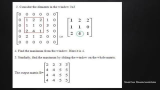
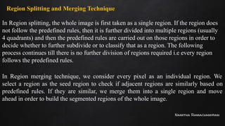
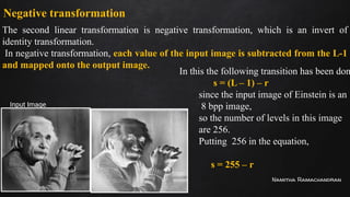
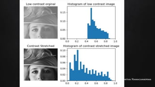
20 30 50 80 100
30 20 80 100 100
20 30 60 10 110
40 30 70 40 100
50 60 80 30 90
Apply standard average filter for pixel at (2,3)
1/16 [30x1+50x2+80x1+20x2+80x4+100x2+30x1+60x2+10x1]
Pixel at (2,3) is 80
1 2 1
2 4 2
1 2 1](https://image.slidesharecdn.com/cg-5-250121101151-98d665d8/85/Computer-graphics-is-drawing-pictures-by-using-computer-aided-methods-and-algorithms-60-320.jpg)