This document presents a novel method for signal separation algorithms that combines Gaussianity and sparsity. It begins with a sparse representation step as preprocessing to address underdetermined mixtures. Then, a Gaussianity-based source separation block is used to estimate the original sources, starting with estimating the mixing matrix. The proposed method was validated using audio signals and the FPICA algorithm. Results showed the original sparse sources and estimated outputs had high signal to interference ratios, demonstrating the quality of separation achieved by the combined Gaussianity and sparsity method.

1. International Journal of Electrical and Computer Engineering (IJECE)
Vol. 7, No. 4, August 2017, pp. 1906~1914
ISSN: 2088-8708, DOI: 10.11591/ijece.v7i4.pp1906-1914  1906
Journal homepage: http://iaesjournal.com/online/index.php/IJECE
A Novel Method based on Gaussianity and Sparsity for Signal
Separation Algorithms
Abouzid Houda, Chakkor Otman
Department of Telecommunications, RSAID Laboratory, National School of Applied Sciences,
Abdelmalek Essaadi University, Tetuan, Morocco
Article Info ABSTRACT
Article history:
Received Jun 9, 2016
Revised Nov 20, 2016
Accepted Dec 11, 2016
Blind source separation is a very known problem which refers to finding the
original sources without the aid of information about the nature of the
sources and the mixing process, to solve this kind of problem having only the
mixtures, it is almost impossible , that why using some assumptions is
needed in somehow according to the differents situations existing in the real
world, for exemple, in laboratory condition, most of tested algorithms works
very fine and having good performence because the nature and the number
of the input signals are almost known apriori and then the mixing process is
well determined for the separation operation. But in fact, the real-life
scenario is much more different and of course the problem is becoming much
more complicated due to the the fact of having the most of the parameters of
the linear equation are unknown. In this paper, we present a novel method
based on Gaussianity and Sparsity for signal separation algorithms where
independent component analysis will be used. The Sparsity as a
preprocessing step, then, as a final step, the Gaussianity based source
separation block has been used to estimate the original sources. To validate
our proposed method, the FPICA algorithm based on BSS technique has
been used.
Keyword:
Gaussianity
Independent Component Analy-
sis (ICA)
Signal Separation Algorithms
Sparse Independent Analysis
Sparsity
Copyright © 2017 Institute of Advanced Engineering and Science.
All rights reserved.
Corresponding Author:
ABOUZID Houda,
Department of Telecommunications,
Abdelmalek Essaadi University,
National School of Applied Sciences, PB 2222 M'hannech, Tetuan, Morocco.
Email: abzdhouda@gmail.com
1. INTRODUCTION
Speech is the most importatnt ways of human communication interaction pickeding up with his
natural michrophones (ears) , therefore when differents speakers are talking in the same time in a room like
in the cocktail party, this human ear listen to mixtures of wanted and unwanted signals.Fortunately, the
human listener is very intelligent in detecting many active sound sources and then he is able to concentrate on
a single source (like a speech of a friend) and ignore the others as a disturbing background noise.However,
this technical operation is not possible for a machine or an humanoid robot because it doesn’t have the brain
like the human, as a consequence , it will get confused having no ability to separate the arrived audio
mixtures and then inderstand the orders. To solve this kind of problems, the blind source separation technique
must be done.
The blind source separation is a very important and recent topic attracted by many reserchers in
differents fields which has been developed and applied to audio signal processing [1]. During the recent years
many studies have been interested to the study of Blind Source Separation (BSS) [2] and more generally to
that of Independent Component Analysis (ICA).This technique is useally based on the hypothesis that the

2. IJECE ISSN: 2088-8708 
A Novel Method based on Gaussianity and Sparsity for Signal Separation Algorithms (Abouzid Houda)
1907
sources are mutually independents.Audio separation method has found its place in many applications, such
as: the cocktail party problem,voice recognition systems ,The noise Suppression for mobile phones or hearing
aids , Medical applications: ECG, EEG,etc.
There are several approches using the BSS technique like:
a. Independent Component Analysis (ICA) method .
b. Time-Frequency masking approach for speech separation .
c. BSS in image separation .
d. Clustering and MMSE-based filtering .
e. Independence .
f. Non-negativity
g. Sparseness
As a result of the central limit theorem, the probability density function of the sum of independent
random variables (or latent variables) is more gaussian than the original random variables. There are many
blind signal separation algorithms in the literature, that uses the gaussianity in order to separate the signals,
where there are many methods for measuring the gaussianity (kurtosis [3], negentrpy [4]) .
In our paper we combine the advantage of the gaussianity and sparsity of the source signal, in order
to separate, recovering and estimating source signals.
To validate our proposed method, we will use audio signals for robotic humanoid applications.
Sparse decompositions techniques will be studied in order to choose a suitable algorithm with better quality
of signal separation.
2. THE PROPOSED METHOD
2.1. Gaussianity based Methods for Signal Separation Algorithms
2.1.1. General Model of BSS
The goal of the Blind signal separation (BSS) is to recover a set of N unknown sources from M
observations resulting from the mixture of these sources through unknown transmission channels. The BSS
problem is present in many real-world applications, such as biomedical, telecommunication and speech [5].
Let a set of the source signals denoted by a vector s =[s1(t),…,sN(t)]T
, the observations or the
recorded signals are x = [x1(t),….,xM(t)]T
. The mixture model for a basic blind signal separation problem is
represented by:
(t) A.s(t)x  (1)
Where A (aij) is an unknown NxN invertible mixing matrix.
In order to study the signal separation methods based on gaussianity, we consider the simple case, where the
number of sources is equal to the number of sensors (N = M), in this case the role of the BSS is to determine
a NxN separating matrix W(wij) such that:
( ) . ( ) . ( )y t W x t G s t  (2)
Where y is an estimate of the source signals .
2.1.2. Independent Component Analysis (ICA)
Independent Component Analysis (ICA) is a famous and classical method used to separate signals
from a linear mixtures of statistical independent component. The principal applications of ICA are blind
signal (sources) separation and feature extraction (Bell and Sejnowski 1996)[6].
All the applications can be formulated in a unified mathematical framework:
We observe n random variables x1, x2, …, xn which are linear combinations of n latent variables s1, s2, …, sn
as:
xi = ai1s1 + ai2s2 + … + ainsn for all i = 1, …, n
Where aij, 1,..., nj  are some real coefficients.
By definition, the sources si are statistically independent. The “latent variables” are the sources si,
which are also called the independent components. They are called “latent” because they cannot directly be
observed or measured. Both the independent components, si, and the mixing coefficients, aij, are not known
and must be determined (or estimated) using only the observed data xi [7].

3.  ISSN: 2088-8708
IJECE Vol. 7, No. 4, August 2017 : 1906 – 1914
1908
The ICA latent variables model is better represented in matrix form. If 1 2
[ , ,..., ]
T
n
S s s s represents
the original, multivariate data that is transformed through some transformation matrix H producing X such
that : X HS .
Then ICA tries to identify an unmixing matrix W such that :
1
W H

 .
So that the resulting matrix Y is: ( )Y WS W HS S S    (since
1
W H

 ).
As we already know, the only thing linear ICA demands is that the original signals 1 2
,s ..., n
s s must
be at any time t statistically independent and the mixing of the sources be linear.
An important preprocessing step before sending the data through the ICA algorithm is whitening.
Whitening is weaker than statistical independence but slightly stronger than uncorrelatedness. The well-
established tool for making sense of high dimensional data by reducing it to a smaller dimension.
Whiteness of a zero-mean random vector, e.g. X , means that its components are uncorrelated and
their variance equals unity. That is, the covariance matrix of X equals the identity matrix I :
{ }
T
E XX I
For our mixed data X , whitening means that we linearly transform it by multiplying with a matrix
(sayV ) such that the resulting matrix Z is white : ( )Z VX V HS H S   .
An important result of whitening process is that the new mixing matrix H , is orthogonal (i.e. its
inverse is equal to its transpose). It is important to note that the whitening (or sphering) process alone does
not ensure statistical independence of X but it plays an important step in the separation process [8].
In order to use the nongaussianity of latent variables, we have to measure the nongaussianity in ICA,
we used some quantitative measure of nongaussianity, like Kurtosis (absolute value) or its square value. They
vanish for a Gaussian variable, and they are positive for most nongaussian random variables [9].
The kurtosis or the fourth-order cumulant of a random variable y is defined for a zero-mean variable
by:
4 2 2
( ) { } 3( { })kurt y E y E y  (3)
If 1
y and 2
y are two independent random variables, we have:
1 2 1 2
( ) ( ) ( )kurt y y kurt y kurt y   (4)
And
4
1 1
( . ) . ( )kurt a y a kurt y (5)
With ( a is a scalar).
The Kurtosis is zero for a Gaussian random variable, and the random variables that have a positive
kurtosis are called super Gaussian (or leptokurtic), and those with negative kurtosis are called sub Gaussian
(or platykurtic).
Negentropy can also be used to measure the nongaussianity.Its defined as follows:
( ) ( ) ( )gauss
J y H y H y  (6)
Where H is the differential entropy of a random vector y defined by:
( ) ( ).log ( )H y f y f y dy  (7)
In the information-theoretic framework, the negentropy is considered as a method to measure the
nongaussianity, and the largest entropy among all the random variables of equal variance is for a Gaussian
variable. The negentropy for a Gaussian variable is zero and always nonnegative [10].
All the solutions proposed for signal separation algorithms, especially those cited in this paper, i.e. the
methods based in the measure of nongaussianity [11], the number of source is equal to the number of sensors,

4. IJECE ISSN: 2088-8708 
A Novel Method based on Gaussianity and Sparsity for Signal Separation Algorithms (Abouzid Houda)
1909
obviously we could have two others situations, the over complete and under complete cases. That why we
propose to use the sparsity, as a solution to separate signals from an underdetermined systems [12].
2.2. Sparsity based methods for Signal Separation Algorithms
Before giving a deep insight about how the sparsity can separate the signals, let’s define the
meaning of a sparse signal.
2.2.1. Definition
The meaning of parsimony is linked to the notion of economy.Thus, a representation of a real vector
is said to be parsimonious if this representation is economical. In other words, there is a more economical
way of describing the vector than giving the value of all its elements. In signal processing, this means that
most of the coefficients are zero, and only a few coefficients have non-zero values. This type of parsimony is
called strict parsimony. The widespread parsimony reflects the fact that the majority of the coefficients have
a low value, while the rest takes quite large values. If we define it in term of Gaussianity, we can say that the
signal is sparse if its marginal distribution has a peak at zero larger than a Gaussian would, or has fatter tails
than those of a Gaussian. The figure below present an exemple of a sparse signal:
Figure 1. Exemple of a sparse signal
The Figure 1 shows that a signal is sparse when its most coefficients are (approximately) zero (the
signal in blue) and that the peaks represent the significant coefficients which constitute the form of the signal.
2.2.2. Applications in Digital Communications
The parsimonious representation of signals has grown significantly over the past decade. This has
made it possible to resolve many problems of signal processing and images such as compression, blind audio
source separation , detection of arrival of sources, or denoising and representation of functions in a basis.
Also a well known applications of the sparsity, is the treatment of inverse problems in
telecommunications exploiting the parsimonious character of the signals to the finite alphabet.
The blind identification of parsimonious channels in SIMO and MIMI-OFDM systems. These
methods have shown performances superior to the methods classical as well as a robustness to the
overestimation of the order of the channel, induced by parsimonious regularization
The sparsity plays an important role resolving the problems referring to themes of identification of
systems (identification of channels), equalization and the identification of parsimonious channels in multi-
sensor systems [13].
2.2.3. Exemple of using Sparsity for Audio Signal Separation
The signals are conventionally represented in the form of a linear transformation of their
coefficients. Conventional signal representation techniques generally use a description of the components on
a basis on which the representation of the signal is unique (Fourier basis, basis of orthogonal wavelets for
example). The Figure 2 shows the representation of a sparse signal in a Fourier basis.
Mathematically, the typical problem of blind signal processing can be formulated as:

5.  ISSN: 2088-8708
IJECE Vol. 7, No. 4, August 2017 : 1906 – 1914
1910
( ) . ( ) ( )x t A s t n t  (8)
With Ais the N M mixing matrix and the noise ( )n t .
So the goal will be to estimate a mixing matrix A and the source signals ( )s t .
Note that, many signals can be sparsely represented using a proper signal dictionary.
The scalar function are called atoms or elements of the dictionary (there are also wavelet-related dictionaries)
which have to be greater than the signal size. Unlike independent component analysis, these elements do not
have to be linearly independent [14].
Figure 2. Representation of a sparse signal using a Fourier basis
3. RESEARCH METHOD
In this paper, our proposed method is based on combining of two principles, one is sparsity’s based
step, it is used as a preprocessing process in order to resolve the problem of the underdetermined mixture,
which is considered one of the great advantages of the sparsity based method for signals separation.
The Gaussianity is used to separate the signals from their mixtures, starting to estimate the mixing
matrix, then moving to proceed a signals separations process using of course the estimated mixing matrix. If
we receive more sources than mixtures, then the problem to estimate the mixing matrix and the estimated
sources is considered as a difficult multivariate optimization problem [15].
The second block is based on gaussianity (or nongaussianity), used as post processing step (or final
step) for the observed signals [16].
The algorithms based on sparsity for signal separation is largely differing from the classical
assumption of the statistical independence of the signals.
4. RESULTS AND DISCUSSION
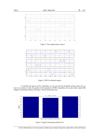
The Figure 3 represents the original sources taht have been taking during the present experiment,
using audio space signals taking from ICALAB, the result seen in the Figure 4, after using the proposed
method:

6. IJECE ISSN: 2088-8708 
A Novel Method based on Gaussianity and Sparsity for Signal Separation Algorithms (Abouzid Houda)
1911
Figure 3. The original sparse sources
Figure 4. FPICA estimated outputs
To describe the precise of ICA algorithm, we use not only the estimated mixing matrix but we
have to use index to show the quality of the separation of FPICA algorithm, this scatter index named SIR
(Signal to Interference Ratio), the Figure 5 below demonstrate that:
Figure 5. Signal to Interference Ratio for S
-4
-2
0
2
4
s1
-4
-2
0
2
4
s2
100 200 300 400 500 600 700 800 900 1000
-4
-2
0
2
4
s3

7.  ISSN: 2088-8708
IJECE Vol. 7, No. 4, August 2017 : 1906 – 1914
1912
Higher values of SIR means that the algorithm performs better for signal separation. As the mean
(SIR) =38.93 dB>20, the performance of the algorithm FPICA is good, and from the plots of the signals we
observe that the extracted signals are similar one by one to the original signal sources.
Figure 6 shows signal to Interference Ratio for A with performance index= 0.007844
Figure 6. Signal to Interference Ratio for A with performance index= 0.007844
The scatter indices of the estimated sources are shown in the Figure 7 below:
Figure 7. The scatter indices of the estimated sources Y
The scatter indices shows the directions of arrival of each signal sources witch the best direction is
the signal which has the most greater indice , here will be the source Y3 having the scatter indice equal to
39.73 dB.

8. IJECE ISSN: 2088-8708 
A Novel Method based on Gaussianity and Sparsity for Signal Separation Algorithms (Abouzid Houda)
1913
5. CONCLUSION
Blind source separation (BSS) is a general signal processing technique, which consists of
recovering, from a finite set of observations recieved by sensors, the contributions of different physical
sources independently from the propagation and without any aid of information a priori on the sources or the
mixing process.
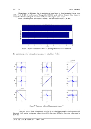
The proposed method has demonstrate improvement performance of signal separation using sparsity
and FPICA algorithm for audio signals. This is could be shown clearly from the figures and the results of
simulation according to the different indices used for testing the quality and the performance of the
separation, which revealed the power of using this two methods together as a common powerful technique.
The human being is able to focus, in the mixture coming from its environment, on one of the sources of
signal that he receives to its both ears. In the case of a weakness of this organ, such as in the hearing
impaired, a DSP improves performance.
The next challenge will be the development of this method in the real time application using digital
signal processing to separate the recieved audio signals for the humanoid robot.
REFERENCES
[1] Kayode F. Akingbade and Isiaka A. Alim, “Separation of Digital Audio Signals using LeastMeanSquare LMS
Adaptive Algorithm”, International Journal of Electrical and Computer Engineering (IJECE), vol.4, no.4,
pp. 557-560, 2014.
[2] Y. Chen, J. Meng, “Study on BSS Algorithm used on Fault Diagnosis of Gearbox”, TELKOMNIKA Indonesian
Journal of Electrical Engineering, vol. 11, no. 6, pp. 2942-2947, 2013.
[3] Rémi Gribonval, Sylvain Lesage, “A Survey of Sparse Component Analysis for Blind Source Separation: Principle,
Perspectives, and new Challenges”, ESANN’2006 proceeding-European Symposium on Artificial Neural
Networks Bruge(Belgium),26-28 April2006,d-side public, ISBN 2-930307-06-4.
[4] Yuanqing Li, Andrzej Cichocki, Shun-ichi Amari, “Sparse Component Analysis for Blind Source Separation with
less Sensors then Sources”, 4th Internatinal Symposium on Independent Component Analysis and Blind Signal
Separation (ICA 2003), April 2003, Nara, Japan.
[5] J.-L. Starck, M. Elad, D. L. Donoho, “Redundant multiscale transforms and their application for Morphological
Component Analysis,”Journal of Advances in Imaging and Electron Physics, vol. 132, pp. 287–348, 2004.
[6] S. Krstulovic, R. Gribonval, “MPTK: Matching Pursuit made Tractable,” in Proc. Int. Conf. Acoust. Speech Signal
Proces.
[7] O. Yilmaz, S.Rickard, ”Blind Separation of Speech Mixtures via Time-Frequency Masking”, IEEE Transaactions
on Signal Processing, vol. 52, no. 7, pp. 1830–1847, Jul. 2004.
[8] P. G. Georgiev, F. Theis, A. Cichocki, “Sparse Component Analysis and blind Source Separation of
underdetermined Mixtures”, IEEE Transactions on Neural Networks, vol. 16, no. 4, pp. 992–996, 2005.
[9] F. J. Theis, A. Jung, C. G. Puntonet, Lang E. W. “Linear geometric ICA: Fundamentals and Algorithms”, Neural
Computation, 15(2): 419-439, February 2003.
[10] A. Ikhlef, D. Le Guennec, “A Simplified Constant Modulus Algorithm for Blind Recovery of MIMO QAM and
PSK Signals: A Criterion with Convergence Analysis”, EURASIP Journal on Wireless Communications and
Networking, vol. 2007, Article ID 90401, 13 pages, 2007. doi :10.1155/2007/90401.
[11] J. F. Cardoso, A. Souloumiac, “Blind Beamforming for Non-Gaussian Signals”, IEE PROCEEDINGS–F, vol. 140,
no. 6, December 1993.
[12] S. Makino, T.-W. Lee, H. Sawada,“Blind Speech Separation”, Springer, 2007.
[13] A. Aissa-El-Bey, “Représentations Parcimonieuses et Applications en Communication Numérique”, Telecom
Bretagne, HDR /Universite de Bretagne Occidentale, 30 Novembre , 2012.
[14] V. Matic, W. Deburchgraeve, “Comparison of ICA Algorithms for ECG Artifact Removal from EEG Signals”,
IEEE-EMBS Benelux Chapter Symposium, 2009.
[15] O. Chakkor, Carlos Garcia Puntonet, Mohammed Essaadi, “A Survey of Signal Separation Algorithms”,
International Journal of Computer Applications, vol. 54, no. 8, 2012.
[16] H. Abouzid, O. Chakkor, “Blind Audio Source Separation: State-of Art”, International Journal of Computer
Applications, vol. 130, no. 4, November 2015.

9.  ISSN: 2088-8708
IJECE Vol. 7, No. 4, August 2017 : 1906 – 1914
1914
BIOGRAPHIES OF AUTHORS
Houda Abouzid was born in Mai 1989 in Tetouan, Morocco, she is a phd student at Abdelmalek
essaadi university, National School of Applied Sciences in Tetouan. She received her degree of
Engineering of telecommunication systems and networks in 2013 at the same scholl. Since 2014,
she has provided several vocational training courses on matlab programming, networks and
embedded systems. She is also a Teacher Vacant at the National School of Applied Sciences
(ENSA-Te). She is the president and member of creation of a telecom generation club at ENSA-Te
since 2016, providing different educational courses and workshops dedicated to all PhD students of
Abdelmalek Essaadi university.
Otman Chakkor was born in November 1977 in Tangier, Morocco. He is a Professor (Head of
Telecommunication Departement) at Abdelmalek Essaadi University, in National School of
Applied Sciences ENSA in Tetuan, Morocco and member of the RSAID Laboratory. He received
his PhD-Thesis from the University of Granada (Spain), Department of Architecture and
Technologies of Computers; Area: Signal processing, He obtained his degree of Electric
Engineering IEEA from Abdelmalek Essaadi University (Morocco) in 1999.