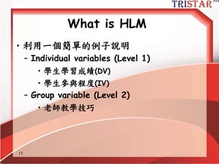
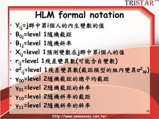
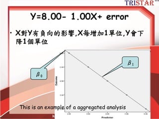
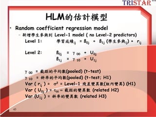
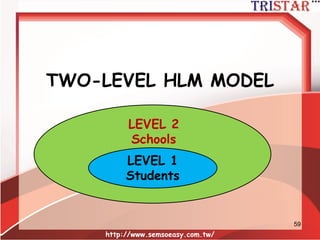
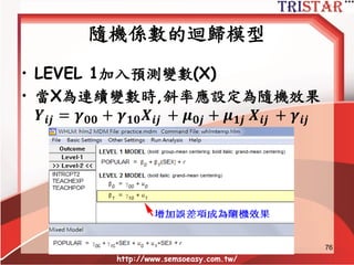
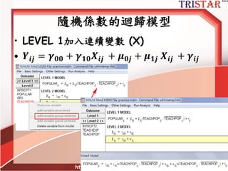
HLM到底在做什麼?
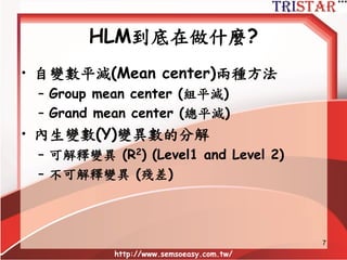
• 自變數平減(Mean center)兩種方法
–Group mean center (組平減)
– Grand mean center (總平減)
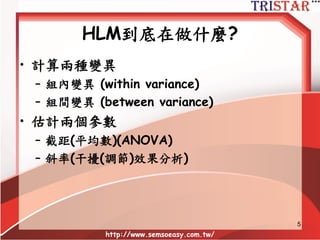
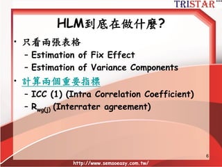
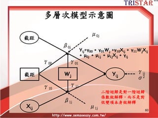
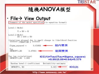
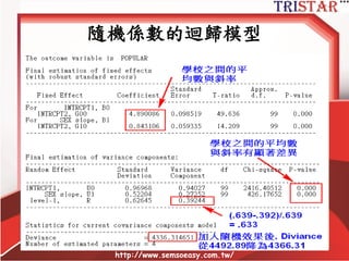
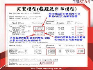
• 內生變數(Y)變異數的分解
– 可解釋變異 (R2) (Level1 and Level 2)
– 不可解釋變異 (殘差)
http://www.semsoeasy.com.tw/
7
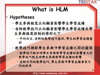
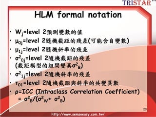
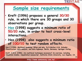
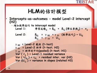
Sample size requirements
•Kreft (1996) proposes a general 30/30
rule, in which there are 30 groups and 30
observations per group.
• Hox (1998) suggests a minimum ratio of
50/20 rule, in order to test cross-level
interactions.
• Hox (1998) also suggests a minimum ratio
of 100/10 to test random effects.
http://www.semsoeasy.com.tw/
36
Hox,J.(1998). Multilevel modeling: When and why. In R.Mathar & M. Schader,
Classification, data analysis, and data highways. Berlin, Germany: Springer-Verlag.
Kreft, I.G.G. (1996). Are multilevel techniques necessary? An overview, including
simulation studies. Unpublished manuscript, California State University, Los Angeles, CA.
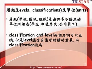
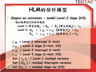
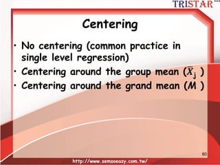
Centering
• No centering(common practice in
single level regression)
• Centering around the group mean ( 𝑿j )
• Centering around the grand mean (M )
http://www.semsoeasy.com.tw/
81
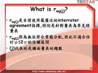
What is rwg(j)?
•rwg(j)是目前使用最廣泛的interrater
agreement指標,特別是針對量表為李克特
量表
• rwg(j)因為無法符合常態分配,因此不適合估
計φ±2σ的信賴區間
• (j)代表的是構面量表的題數
http://www.semsoeasy.com.tw/
90
91.
91
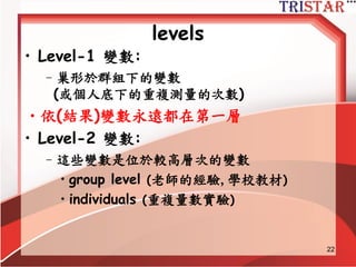
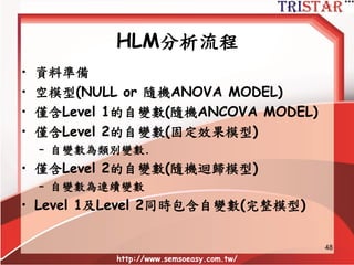
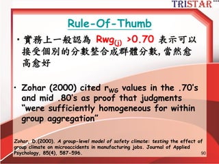
Rule-Of-Thumb
•實務上一般認為 Rwg(j) >0.70表示可以
接受個別的分數整合成群體分數,當然愈
高愈好
• Zohar (2000) cited rWG values in the .70’s
and mid .80’s as proof that judgments
“were sufficiently homogeneous for within
group aggregation”
Zohar, D.(2000). A group-level model of safety climate: testing the effect of
group climate on microaccidents in manufacturing jobs. Journal of Applied
Psychology, 85(4), 587-596.
92.
How to calculaterwg(j)?
http://www.semsoeasy.com.tw/
92
James L R, Demaree R G, Wolf G.(1993). Rwg: An Assessment of within-
Group Interrater Agreement. Journal of Applied Psychology.78, 306-309.
94
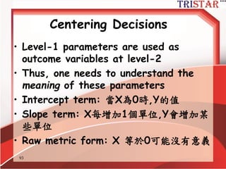
Centering Decisions
• Level-1parameters are used as
outcome variables at level-2
• Thus, one needs to understand the
meaning of these parameters
• Intercept: 當X為0時,Y的期望值
• Slope: X每增加1個單位,Y期望增加某些單
位
• Raw metric form: X等於0可能沒有意義
95.
95
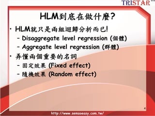
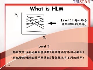
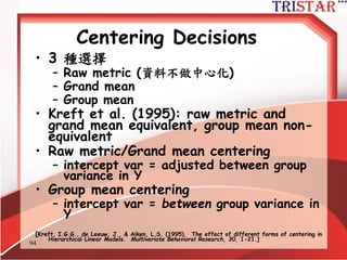
Centering Decisions
• 3種選擇
– Raw metric (資料不做中心化)
– Grand mean
– Group mean
• Kreft et al. (1995): raw metric and
grand mean equivalent, group mean non-
equivalent
• Raw metric/Grand mean centering
– intercept var = adjusted between group
variance in Y
• Group mean centering
– intercept var = between group variance in
Y
[Kreft, I.G.G., de Leeuw, J., & Aiken, L.S. (1995). The effect of different forms of centering in
Hierarchical Linear Models. Multivariate Behavioral Research, 30, 1-21.]
96.
96
Centering Decisions
• 重點是…
–Grand mean centering and/or raw
metric estimate incremental models
• Controls for variance in level-1 variables
prior to assessing level-2 variables
– Group mean centering
• Does NOT estimate incremental models
– Does not control for level-1 variance
before assessing level-1 variables
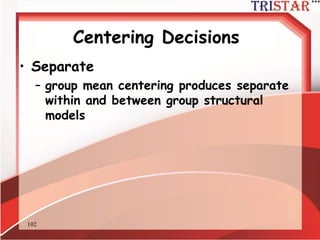
– Separately estimates with group
regression and between group
regression
97.
97
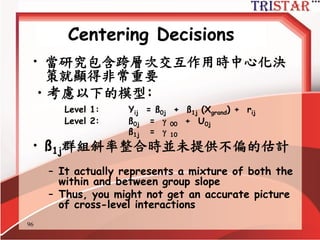
Centering Decisions
• 當研究包含跨層次交互作用時中心化決
策就顯得非常重要
•考慮以下的模型:
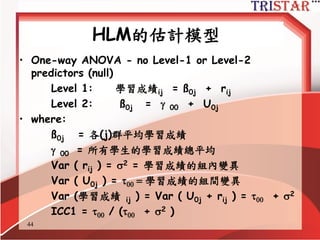
Level1: Yij = ß0j + ß1j (Xgrand) + rij
Level 2: ß0j = 00 + U0j
ß1j = 10
• ß1j群組斜率整合時並未提供不偏的估計
– It actually represents a mixture of both the
within and between group slope
– Thus, you might not get an accurate picture
of cross-level interactions
98.
98
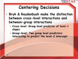
Centering Decisions
• Bryk& Raudenbush make the distinction
between cross-level interactions and
between-group interactions
– Cross-level: Group level predictor of level-1
slopes
– Group-level: Two group level predictors
interacting to predict the level-2 intercept
99.
99
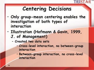
Centering Decisions
• Onlygroup-mean centering enables the
investigation of both types of
interaction
• Illustration (Hofmann & Gavin, 1999,
J. of Management)
– Created two data sets
• Cross-level interaction, no between-group
interaction
• Between-group interaction, no cross-level
interaction
100.
100
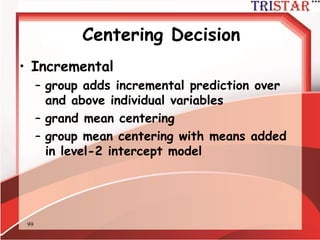
Centering Decision
• Incremental
–group adds incremental prediction over
and above individual variables
– grand mean centering
– group mean centering with means added
in level-2 intercept model
101.
101
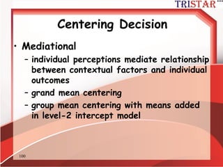
Centering Decision
• Mediational
–individual perceptions mediate relationship
between contextual factors and individual
outcomes
– grand mean centering
– group mean centering with means added
in level-2 intercept model
102.
102
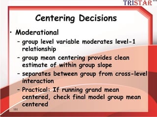
Centering Decisions
• Moderational
–group level variable moderates level-1
relationship
– group mean centering provides clean
estimate of within group slope
– separates between group from cross-level
interaction
– Practical: If running grand mean
centered, check final model group mean
centered
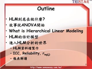

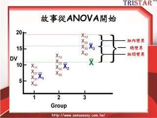
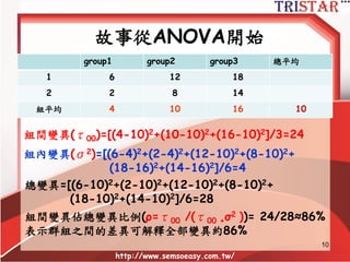
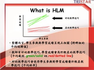
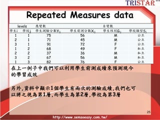
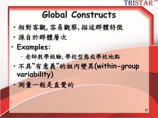
![故事從ANOVA開始
group1 group2 group3 總平均
1 6 12 18
2 2 8 14
組平均 4 10 16 10
http://www.semsoeasy.com.tw/
11
組間變異(τ00)=[(4-10)2+(10-10)2+(16-10)2]/3=24
組內變異(σ2)=[(6-4)2+(2-4)2+(12-10)2+(8-10)2+
(18-16)2+(14-16)2]/6=4
總變異=[(6-10)2+(2-10)2+(12-10)2+(8-10)2+
(18-10)2+(14-10)2]/6=28
組間變異佔總變異比例(ρ=τ00 /(τ00 +σ2 ))= 24/28≈86%
表示群組之間的差異可解釋全部變異約86%](https://image.slidesharecdn.com/hlm-150207232658-conversion-gate01/85/HLM-11-320.jpg)
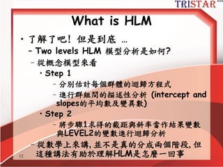
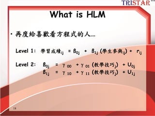
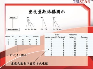


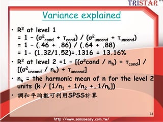
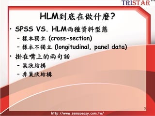
![Variance explained
• R2 at level 1
= 1 – (σ2
cond + τcond) / (σ2
uncond + τuncond)
= 1 – (.46 + .86) / (.64 + .88)
= 1- (1.32/1.52)=.1316 = 13.16%
• R2 at level 2 =1 – [(σ2cond / nh) + τcond] /
[(σ2
uncond / nh) + τuncond]
• nh = the harmonic mean of n for the level 2
units (k / [1/n1 + 1/n2 +…1/nk])
• 調和平均數可利用SPSS計算
http://www.semsoeasy.com.tw/
75](https://image.slidesharecdn.com/hlm-150207232658-conversion-gate01/85/HLM-75-320.jpg)

![95
Centering Decisions
• 3 種選擇
– Raw metric (資料不做中心化)
– Grand mean
– Group mean
• Kreft et al. (1995): raw metric and
grand mean equivalent, group mean non-
equivalent
• Raw metric/Grand mean centering
– intercept var = adjusted between group
variance in Y
• Group mean centering
– intercept var = between group variance in
Y
[Kreft, I.G.G., de Leeuw, J., & Aiken, L.S. (1995). The effect of different forms of centering in
Hierarchical Linear Models. Multivariate Behavioral Research, 30, 1-21.]](https://image.slidesharecdn.com/hlm-150207232658-conversion-gate01/85/HLM-95-320.jpg)