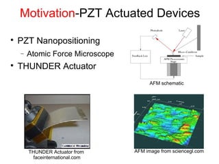
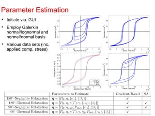
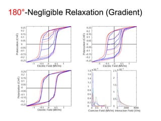
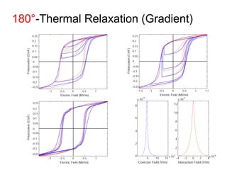
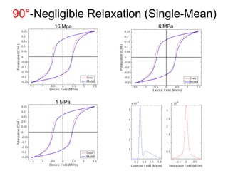
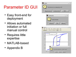
This document outlines a final oral exam presentation on high-speed parameter estimation for a homogenized energy model, discussing applications, motivation, employed models, and parameter estimation techniques. It details results using gradient-based and stochastic searches for PZT data, as well as future work directions. The presentation highlights the development of a GUI for parameter estimation, significant improvements in computational efficiency, and the successful implementation of new density formulations and estimation methodologies.

1. High Speed Parameter Estimation
for a Homogenized Energy Model
Final Oral Exam
Jon M. Ernstberger
Advisor: Ralph C. Smith
June 23, 2008

2. Presentation Outline

Applications

Motivation

Employed Models

Past density formulations

Initial estimate techniques

Galerkin expansion HEM formulation

Incorporated Temperature dependence

Results using gradient-based and stochastic searches to PZT data

Future Work

3. Applications
• Jet Engine Chevrons
• 4 dB engine noise reduction
• 3 dB reduction occurs if you
turn off a jet engine
• Bio-medical applications (SMAs)
• Heart stents
• Reconstructive surgery
• Energy harvesting
• DARPA Initiative
• Recharge devices
• THUNDER
• Pumps
• Valves
Courtesy of boeing.com
boeing.com
From crucibleresearch.com

4. Motivation-Active Machining System
• ETREMA Products, Inc.
• Active Mat. Terfenol-D
• High-Speed Milling (4,000
RPM)
Courtesy of http://www.etrema-usa.com/

5. Motivation-PZT Actuated Devices

PZT Nanopositioning
− Atomic Force Microscope

THUNDER Actuator
AFM image from sciencegl.com
AFM schematic
THUNDER Actuator from
faceinternational.com

6. Energies-Ferromagnetic
Gibbs EnergyHelmholtz Energy
w. neg. thermal relaxation
Local Hysteron from

7. Thermal Relaxation
Moment Fraction Evolution:
Local Avg. Magnetization:
Expected Magnetization:
Switching Likelihood:
Boltzmann Relation:

8. Homogenized Energy Model
Subject to:
Where:

9. Helmholtz Energy
Gibbs Energy
Local Polarization
Energies-Ferroelectric

10. 180° Switching-Thermal Relaxation
Boltzmann Relation
Switching Likelihood
Dipole Fraction Evolution
Expected Polarization
Local Average Polarization

11. 90° Switching-Energies/Local Relations
Helmholtz Energies
Gibbs Energy
Local Polarization 90°-Switch due to compressive stress

12. 90° Switching-Thermal Relaxation
Boltzmann Relation
Switching Likelihood
Dipole Fraction Evolution
Expected Polarization
Local Average Polarization

13. Homogenized Energy Model-Ferroelectrics
 Four Kernels
− 180°-Switching
 Negligible relaxation
 Thermal relaxation
− 90°-Switching
 Negligible relaxation
 Thermal relaxation
 Density Behaviors
− Exponential decay
− Interaction field symmetry
− Positive coercive field
domain
 Quadrature Decomposition

14. Temperature Dependence
Using a Helmholtz Energy which incorporates Temperature
from which are yielded
through the relation

15. Lumped Rod Model
Balance rod forces σA with restoring mechanism
or

16. Density Choice-Normal/Lognormal
Runtime 52.90 seconds
100 Hz 200 Hz
300 Hz 500 Hz

17. Parameter ID-Initial Estimate (E-P)
Remanence
Susceptibility
Density Parameters

Standard deviations

Coercive field mean
(a)
(b)

18. Parameter ID-Initial Estimate (E-P)

19. Parameter ID-Initial Estimate/Strain
Recall

Ignore Kelvin-Voigt damping, magnetostriction, and derivative terms

Presume no applied stress, knowledge of remanence and Young's modulus,
and simple magnetization

Determine suspectibility and piezomagnetization
coefficients

Determine coercive field mean and standard deviation

Determine interaction field standard deviation

20. Parameter ID-Initial Estimate/Strain

Simplified model embedded into a “point-click” GUI

(a) 100 Hz, (b) 200 Hz, (c ) 300 Hz, and (d) 500 Hz

21. Constraints
Density points to estimate

22. Densities-Constrained General Densities

Best fit

10 quadrature
intervals per density

68 parameters to
estimate

Runtime 969.43
seconds
100 Hz 200 Hz
300 Hz 500 Hz

23. Densities-Galerkin Expansions
Use Galerkin expansion approximate to general densities
Advantages: 1. Smaller parameter space (8+3(N+1)/2 vs. 8+6N)
2. Decrease in runtime in comparison to general density
Disdvantages: 1. Fit will not be as good as general density fit
2. Still requires density constraints for physical behavior

24. Densities-SQP/SQP Linear expansion
100 Hz 200 Hz
300 Hz 500 Hz
•N=8 Intervals
•4 Pt. Gauss. Quad.
•Linear Expansion
•2000 SQP Fcn Evals
•Runtime: 164.7s

25. Galerkin Normal/Lognormal Basis
– Normally distributed basis elements for interaction field density
– Lognormally distributed basis elements for the coercive field density
– Removes decay constraints

26. Densities: Galerkin normal/lognormal
w. single mean

Runtime 250 seconds

10 quadrature intervals

5 interaction field
bases

7 coercive field bases
100 Hz 200 Hz
300 Hz 500 Hz

27. Densities: Galerkin normal/lognormal
w. multiple means

Runtime 244.7
seconds

10 quadrature intervals

5 interaction field
bases

9 coercive field bases
(3 std. devs, 3 means)

Lower residual than
single mean
100 Hz 200 Hz100 Hz
300 Hz 500 Hz

28. Temperature Dependence
Top: Terfenol-D Data M vs. H data taken at 292 and 363 K.
Bottom: Fits to data using estimated parameters.

29. 
Initiate via. GUI

Employ Galerkin
normal/lognormal and
normal/normal basis

Various data sets (inc.
applied comp. stress)
Parameter Estimation

30. 180°-Negligible Relaxation (Gradient)

31. 180°-Thermal Relaxation (Gradient)

32. 90°-Negligible Relaxation (Gradient)

33. 90°-Negligible Relaxation (Single-Mean)
16 Mpa 8 MPa
1 MPa

34. 90°-Negligible Relaxation (Multi-Mean)
16 MPa 8 MPa
1 MPa

35. 180°-Thermal Relaxation (SA)

36. 90°-Negligible Relaxation (SA)
Galerkin normal/normal basis

37. 90°-Negligible Relaxation
Applied Compressive Stress (SA)
16 MPa 8 MPa
1 MPa

38. Conclusions

Augmented previous density formulations to
generate more physical approximates

Eased estimation computation load w. linear and
cubic Galerkin expansion formulation of the HEM

Successfully implemented Galerkin
normal/lognormal (normal/normal) basis

Tools to determine initial parameter estimates for
field-polarization and field-strain data.

Reduced parameter estimation runtime for the AMS
to about 4 minutes

Performed parameter estimation to Terfenol-D/AMS
data with gradient-based and stochastic searches

39. Conclusions (2)

Achieved accurate PZT parameter estimates
employing for kernels with 90° and 180°-switching
(including data w. applied compressive stress)

Validated toolset for initial estimates

Estimated parameters with gradient-based routines
and simulated annealing

Showed dissipativity of the HEM

Generated a full GUI for the parameter estimation
process

40. Future Work

Ferroelastic model with thermal relaxation

Combination Galerkin normal/lognormal basis
w. Temperature Dep.

Terfenol-D/PZT data to fit.

Hybrid gradient/stochastic searches

Estimation for SMA model

41. References

48. 
If a system is dissipative, it loses energy.

“The energy at final time is less than or equal to initial
energy plus input energy.”

Showed dissipativity of
− HEM with negligible thermal relaxation for supply rates
and
− HEM with thermal relaxation for same supply rates

Statement of stability and helps design controllers
Dissipativity of HEM
HM MH 

49. Parameter ID GUI

Easy front-end for
deployment

Allows automated
initiation or full
manual control

Requires little
expertise

MATLAB-based

Appendix B