Robert D. Falgout and Panayot Vassilevski
Center for Applied Scientific Computing
Lawrence Livermore National Laboratory
Germany
June, 2003
On Generalizing the AMG
Framework
RDF 2CASC
Outline
AMG / AMGe framework background
New Measures and Convergence Theory
Building Interpolation
Compatible Relaxation
Examples
Conclusions and future directions
RDF 3CASC
AMG / AMGe Framework
AMGe heuristic is based on multigrid theory:
interpolation must reproduce a mode up to the same
accuracy as the size of the associated eigenvalue
Bound a measure (weak approximation property):
Localize the measure to build AMGe components
Several variants developed: E-Free, Spectral
Based on pointwise relaxation
Assumes coarse grid is a subset of fine grid
IPQ
eeA
eQIeQI
A =;
,
)−(,)−(
0
RDF 4CASC
We are generalizing our AMG framework
to address new problem classes
Maxwell and Helmholtz problems have huge near
null spaces and require more than pointwise
smoothing to achieve optimality in multigrid
Our new theory allows for any type of smoother, and
also works for a variety of coarsening approaches
(e.g., vertex-based, cell-based, agglomeration)
Paper submitted
Model of a section of the Next
Linear Collider structure
Resonant frequencies in
a Helmholtz Application
RDF 5CASC
Preliminaries…
Consider solving the linear system
Consider smoothers of the form
where we assume that (M+MT
− A) is SPD (necessary
& sufficient condition for convergence)
Note: M may be symmetric or nonsymmetric
Smoother error propagation
fuA =
rMuu kkk
−
+
1
1 +=
ek + 1 = ( I − M − 1
A) ek
RDF 6CASC
Preliminaries continued…
Let P : ℜnc → ℜn
be interpolation (prolongation)
Let R : ℜn
→ ℜnc be some “restriction” operator
— Note that R is not the MG restriction operator
— The form of R will be important later
Define Q : ℜn
→ ℜn
to be a projection onto range(P);
hence Q=PR such that RP=I
RDF 7CASC
Two new measures
First measure:
Second measure: Define (M) ≡ ½(M+MT
) , then
Measure µσ is the analogue to the AMGe measure
,
)−(,)−()−+(
=),(µ
eeA
eQIeQIMAMMM
eQ
TT − 1
,
)−(,)−()(σ
=),(µσ
eeA
eQIeQIM
eQ
RDF 8CASC
First measure and MG convergence
Theorem: Assume that the following holds for some
constant K:
Then, 2-level MG converges uniformly:
Here, QA = P(PT
AP)-1
PT
A is the A-orthogonal projector
onto range(P)
As in AMGe, we could try to directly localize this
new measure to help us build AMG algorithms
But, we will take a different approach
µ( Q,e) ≤ K ∀e∈ℜn
 {0}
−≤)−()−( eeQIAMI
/
−
21
11
AKA
A 1
RDF 9CASC
Second measure and MG convergence
Bounding µσ also implies uniform convergence…
Lemma: Assume that (M+MT
− A) is SPD. Then,
where ∆ ≥ 1 measures the deviation of M from (M)
and where 0 < ω ≡ λmax(σ(M)-1A) < 2 .
Must insure “good” constants
— in particular, ω « 2
),(µ
ω−
∆
≤),(µ eQeQ
2
2
σ
Mv,w ≤ ∆ σ( M) v,v
1/2
σ( M) w,w
1/2
RDF 10CASC
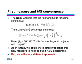
General notions of C-pts & F-pts
Recall the projection Q=PR, with RP=I
We now fix R so that it does not depend on P
— Defines the coarse-grid variables, uc = Ru
— Recall that R=[ 0, I ] (PT
=[ WT
, I ]T
) for AMGe; i.e., the coarse-
grid variables were a subset of the fine grid
— C-pt analogue
Define S : ℜns → ℜn
s.t. ns= n− nc and RS = 0
— Think of range(S) as the “smoother space”, i.e., the space on
which the smoother must be effective
— Note that S is not unique
— F-pt analogue
S and RT
define an orthogonal decomposition of ℜn
;
any vector e can be written as e = Ses+ RT
ec
RDF 11CASC
The Min-max Problem
Consider the following base measure, where X is any
SPD matrix:
Theorem: Define
The arg min satisfies ST
AP* = 0 and the minimum is
We will call P* the optimal interpolation operator
),(µ≡µ XX
≠
∗ xamnim
eP 0
eRP
))()((λ=µX
−−∗ 11
nim SASSXS TT
,
)−(,)−(
≡),(µX
eeA
eQIeQIX
eQ
RDF 12CASC
The Min-max Problem… and AMGe
The optimal interpolation has the general form:
For AMGe, the coarse-grid variables are a subset of
the fine grid:
Hence,
I
RASSASRSP
−
∗
)()(−=
TTT
T
1
I
S
I
W
PIR =;=;=
0
0
A
A
I
AA
P ∗
−
∗
)(λ
=µ,
−
=
ff
cfff
nim
1
X
RDF 13CASC
The Min-max Problem… Spectral AMGe
and Smoothed Aggregation (SA)
For Spectral AMGe and SA, the coarse-grid variables
are coefficients of basis functions:
where the pi are orthonormal eigenvectors of A with
eigenvalues λ1 ≤ … ≤ λn . Hence,
The optimal interpolation can also be viewed as a
“smoothed” tentative prolongator
RASSASSIP −
∗ ))(−(= TTT 1
ppSIPRppR ncc
T
,...,=,=,,...,= 11 +
RP
+
∗
∗
λ
λ
=µ,=
c
nT
X
1
RDF 14CASC
The new theory separates construction of
coarse-grid correction into two parts
The following measures the ability of a given coarse
grid Ωc to represent algebraically smooth error:
Theorem: (1) Assume that µ* ≤ K for some constant K.
(2) Assume that any one of the following holds for η ≥ 1:
Then, µ(PR, e) ≤ ηK, ∀e.
(1) insures coarse grid quality – use CR
(2) insures interpolation quality – necessary condition
that does not depend on relaxation!
),(µ≡µ
≠
∗ xamnim
eP 0
eRP
eeeAeQeQA ∀,,η≤,
eeeAeQIeQIA ∀,,η≤)−(,)−(
eeeSeSAePePAeSePA scssccsc ,∀,,,)η−(≤, 12
1 −
RDF 15CASC
CR is an efficient method for measuring
the quality of the set of coarse variables
CR (Brandt, 2000) is a modified relaxation scheme
that keeps the coarse-level variables, Ru, invariant
We have defined several variants of CR, and shown
that fast converging CR implies a good coarse grid:
Hence, CR can be used as a tool to efficiently
measure the quality of a coarse grid!
General idea: If CR is slow to converge, either increase
the size of the coarse grid or modify relaxation
F-relaxation is a specific instance of CR
ρ−ω−
∆
≤µ ∗
2
1
1
2 rc
RDF 16CASC
We can use CR to choose the coarse grid
To check convergence of CR, relax on the equation
and monitor pointwise convergence to 0
CR coarsening algorithm:
xA ff = 0
fotestnednepedni
speewsnoitaxalerelbitapmocoD
elihW
ezilaitinI
CFUCC
xxiU
U
CFCU
−Ω=;}{∪=
}θ>|/|:{=
ν
∅≠
−Ω=;∅=;Ω=
ii
−νν 1
RDF 17CASC
Using CR to choose the coarse grid
Initialize U-pts
Do CR and redefine
U-pts as points
slow to converge
Select new C-pts as
indep. set over U
RDF 18CASC
Using CR to choose the coarse grid
Initialize U-pts
Do CR and redefine
U-pts as points
slow to converge
Select new C-pts as
indep. set over U
RDF 19CASC
Using CR to choose the coarse grid
Initialize U-pts
Do CR and redefine
U-pts as points
slow to converge
Select new C-pts as
indep. set over U
RDF 20CASC
Using CR to choose the coarse grid
Initialize U-pts
Do CR and redefine
U-pts as points
slow to converge
Select new C-pts as
indep. set over U
RDF 21CASC
Using CR to choose the coarse grid
Initialize U-pts
Do CR and redefine
U-pts as points
slow to converge
Select new C-pts as
indep. set over U
RDF 22CASC
CR based on matrix splittings
Theorem: Assume that (M+MT
− A) is SPD. Then,
where ∆ and ω are as before, and ρs = (I − Ms
-1
As) As
.
Fast converging CR implies good coarse grid
If relaxation is based on a splitting A = M − N, then M
is explicitly available, and CR is probably feasible
ek + 1 = ( I − Ms
− 1
As) ek; Ms = ST
MS; As = ST
AS
≤µ
ρ−ω−
∆∗
2
1
1
2 s
RDF 23CASC
CR based on additive subspace methods
Consider the following additive method:
where Ii : ℜni → ℜn
and ℜn
= ∪i range(Ii).
Define full rank normalized operators Si and Ri
T
s.t.
range(Si) = range(Ii
T
S) and range(Ri
T
) = range(Ii
T
RT
)
The Ii must be chosen so that Ri Si=0
Then an additive CR is given by
Same theoretical result as before, but with ∆ = 1
IIAIIMAMI )(=;− −−− 111 T
ii
T
iii
SIIIIAIISMAMI =;)(=;− iiis
T
isis
T
isis
T
ircsrc ,,
−
,,,
−− 111
RDF 24CASC
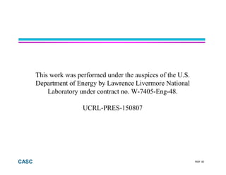
Compatible Additive Schwarz is natural
when R=[ 0, I ]
Just remove coarse-grid points from subdomains
It is clear that Ri Si=0 for any choice of Ii
Additive Schwarz CR Additive Schwarz
RDF 25CASC
More general form of CR
Here, S must be normalized so that ST
S = I
This variant of CR is always computable
Theoretical result currently requires SPD smoother,
M, and involves an additional constant:
where γ∈[0,1) satisfies
SASAeASMSIe T
sks
T
k
−
+
1
1 =;))(−(=
≤µ
ρ−γ−ω−
∗
1
1
1
1
2
1
2 s
vvvRvRMvSvSMvRvSM csc
T
c
T
ssc
T
s ,∀;,,γ≤,
2121 //
RDF 26CASC
Another general form of CR (due to
Brandt and Livne)
As before, S must be normalized so that ST
S = I
This variant of CR is also always computable
Theoretical result is similar, but weaker:
≤µ
)ρ−(γ−ω−
∗
1
1
1
2
2
1
22
s
eSAMISeSAMSIe k
T
k
T
k
−−
+
11
1 )−(=)−(=
RDF 27CASC
Anisotropic Diffusion Example
Dirichlet BC’s and ε∈(0,1]
Piecewise linear elts on triangles
Standard coarsening, i.e., S = [ I, 0 ]T
The spectrum of the CR iteration matrix satisfies
Linear interpolation satisfies, with η = 2,
=−ε− fuu yyxx
,−∈)−(λ AMI ss
ε+
ε
ε+
ε−
22
1
eeeAeQeQA ∀,,η≤,
RDF 28CASC
Anisotropic Diffusion Example –
leveraging previous work
Consider the AMGe measure
It is easy to show that η ≥ A / ε
As mentioned earlier, this implies
But the AMGe method produces linear interpolation;
it is just unable to judge its quality in this setting
(i.e., when using line relaxation)
A ( I − Q) e
2
≤ η Ae, e
eeeAeQIeQIA ∀,,η≤)−(,)−(
RDF 29CASC
Conclusions and Future Directions
We have developed a more general theoretical
framework for AMG methods
— Allows for any type of smoother
— Allows for a variety of coarsening approaches (e.g., vertex-
based, cell-based, agglomeration)
The theory separates construction of coarse-grid
correction into two parts:
— Insuring the quality of the coarse grid via CR
— Insuring the quality of interpolation for the given coarse grid
(leverages earlier work)
We have defined several variants of CR
Will explore further the use of CR in practice
Choosing / modifying smoothers automatically?
RDF 30CASC
This work was performed under the auspices of the U.S.
Department of Energy by Lawrence Livermore National
Laboratory under contract no. W-7405-Eng-48.
UCRL-PRES-150807

Germany2003 gamg

  • 1.
    Robert D. Falgoutand Panayot Vassilevski Center for Applied Scientific Computing Lawrence Livermore National Laboratory Germany June, 2003 On Generalizing the AMG Framework
  • 2.
    RDF 2CASC Outline AMG /AMGe framework background New Measures and Convergence Theory Building Interpolation Compatible Relaxation Examples Conclusions and future directions
  • 3.
    RDF 3CASC AMG /AMGe Framework AMGe heuristic is based on multigrid theory: interpolation must reproduce a mode up to the same accuracy as the size of the associated eigenvalue Bound a measure (weak approximation property): Localize the measure to build AMGe components Several variants developed: E-Free, Spectral Based on pointwise relaxation Assumes coarse grid is a subset of fine grid IPQ eeA eQIeQI A =; , )−(,)−( 0
  • 4.
    RDF 4CASC We aregeneralizing our AMG framework to address new problem classes Maxwell and Helmholtz problems have huge near null spaces and require more than pointwise smoothing to achieve optimality in multigrid Our new theory allows for any type of smoother, and also works for a variety of coarsening approaches (e.g., vertex-based, cell-based, agglomeration) Paper submitted Model of a section of the Next Linear Collider structure Resonant frequencies in a Helmholtz Application
  • 5.
    RDF 5CASC Preliminaries… Consider solvingthe linear system Consider smoothers of the form where we assume that (M+MT − A) is SPD (necessary & sufficient condition for convergence) Note: M may be symmetric or nonsymmetric Smoother error propagation fuA = rMuu kkk − + 1 1 += ek + 1 = ( I − M − 1 A) ek
  • 6.
    RDF 6CASC Preliminaries continued… LetP : ℜnc → ℜn be interpolation (prolongation) Let R : ℜn → ℜnc be some “restriction” operator — Note that R is not the MG restriction operator — The form of R will be important later Define Q : ℜn → ℜn to be a projection onto range(P); hence Q=PR such that RP=I
  • 7.
    RDF 7CASC Two newmeasures First measure: Second measure: Define (M) ≡ ½(M+MT ) , then Measure µσ is the analogue to the AMGe measure , )−(,)−()−+( =),(µ eeA eQIeQIMAMMM eQ TT − 1 , )−(,)−()(σ =),(µσ eeA eQIeQIM eQ
  • 8.
    RDF 8CASC First measureand MG convergence Theorem: Assume that the following holds for some constant K: Then, 2-level MG converges uniformly: Here, QA = P(PT AP)-1 PT A is the A-orthogonal projector onto range(P) As in AMGe, we could try to directly localize this new measure to help us build AMG algorithms But, we will take a different approach µ( Q,e) ≤ K ∀e∈ℜn {0} −≤)−()−( eeQIAMI / − 21 11 AKA A 1
  • 9.
    RDF 9CASC Second measureand MG convergence Bounding µσ also implies uniform convergence… Lemma: Assume that (M+MT − A) is SPD. Then, where ∆ ≥ 1 measures the deviation of M from (M) and where 0 < ω ≡ λmax(σ(M)-1A) < 2 . Must insure “good” constants — in particular, ω « 2 ),(µ ω− ∆ ≤),(µ eQeQ 2 2 σ Mv,w ≤ ∆ σ( M) v,v 1/2 σ( M) w,w 1/2
  • 10.
    RDF 10CASC General notionsof C-pts & F-pts Recall the projection Q=PR, with RP=I We now fix R so that it does not depend on P — Defines the coarse-grid variables, uc = Ru — Recall that R=[ 0, I ] (PT =[ WT , I ]T ) for AMGe; i.e., the coarse- grid variables were a subset of the fine grid — C-pt analogue Define S : ℜns → ℜn s.t. ns= n− nc and RS = 0 — Think of range(S) as the “smoother space”, i.e., the space on which the smoother must be effective — Note that S is not unique — F-pt analogue S and RT define an orthogonal decomposition of ℜn ; any vector e can be written as e = Ses+ RT ec
  • 11.
    RDF 11CASC The Min-maxProblem Consider the following base measure, where X is any SPD matrix: Theorem: Define The arg min satisfies ST AP* = 0 and the minimum is We will call P* the optimal interpolation operator ),(µ≡µ XX ≠ ∗ xamnim eP 0 eRP ))()((λ=µX −−∗ 11 nim SASSXS TT , )−(,)−( ≡),(µX eeA eQIeQIX eQ
  • 12.
    RDF 12CASC The Min-maxProblem… and AMGe The optimal interpolation has the general form: For AMGe, the coarse-grid variables are a subset of the fine grid: Hence, I RASSASRSP − ∗ )()(−= TTT T 1 I S I W PIR =;=;= 0 0 A A I AA P ∗ − ∗ )(λ =µ, − = ff cfff nim 1 X
  • 13.
    RDF 13CASC The Min-maxProblem… Spectral AMGe and Smoothed Aggregation (SA) For Spectral AMGe and SA, the coarse-grid variables are coefficients of basis functions: where the pi are orthonormal eigenvectors of A with eigenvalues λ1 ≤ … ≤ λn . Hence, The optimal interpolation can also be viewed as a “smoothed” tentative prolongator RASSASSIP − ∗ ))(−(= TTT 1 ppSIPRppR ncc T ,...,=,=,,...,= 11 + RP + ∗ ∗ λ λ =µ,= c nT X 1
  • 14.
    RDF 14CASC The newtheory separates construction of coarse-grid correction into two parts The following measures the ability of a given coarse grid Ωc to represent algebraically smooth error: Theorem: (1) Assume that µ* ≤ K for some constant K. (2) Assume that any one of the following holds for η ≥ 1: Then, µ(PR, e) ≤ ηK, ∀e. (1) insures coarse grid quality – use CR (2) insures interpolation quality – necessary condition that does not depend on relaxation! ),(µ≡µ ≠ ∗ xamnim eP 0 eRP eeeAeQeQA ∀,,η≤, eeeAeQIeQIA ∀,,η≤)−(,)−( eeeSeSAePePAeSePA scssccsc ,∀,,,)η−(≤, 12 1 −
  • 15.
    RDF 15CASC CR isan efficient method for measuring the quality of the set of coarse variables CR (Brandt, 2000) is a modified relaxation scheme that keeps the coarse-level variables, Ru, invariant We have defined several variants of CR, and shown that fast converging CR implies a good coarse grid: Hence, CR can be used as a tool to efficiently measure the quality of a coarse grid! General idea: If CR is slow to converge, either increase the size of the coarse grid or modify relaxation F-relaxation is a specific instance of CR ρ−ω− ∆ ≤µ ∗ 2 1 1 2 rc
  • 16.
    RDF 16CASC We canuse CR to choose the coarse grid To check convergence of CR, relax on the equation and monitor pointwise convergence to 0 CR coarsening algorithm: xA ff = 0 fotestnednepedni speewsnoitaxalerelbitapmocoD elihW ezilaitinI CFUCC xxiU U CFCU −Ω=;}{∪= }θ>|/|:{= ν ∅≠ −Ω=;∅=;Ω= ii −νν 1
  • 17.
    RDF 17CASC Using CRto choose the coarse grid Initialize U-pts Do CR and redefine U-pts as points slow to converge Select new C-pts as indep. set over U
  • 18.
    RDF 18CASC Using CRto choose the coarse grid Initialize U-pts Do CR and redefine U-pts as points slow to converge Select new C-pts as indep. set over U
  • 19.
    RDF 19CASC Using CRto choose the coarse grid Initialize U-pts Do CR and redefine U-pts as points slow to converge Select new C-pts as indep. set over U
  • 20.
    RDF 20CASC Using CRto choose the coarse grid Initialize U-pts Do CR and redefine U-pts as points slow to converge Select new C-pts as indep. set over U
  • 21.
    RDF 21CASC Using CRto choose the coarse grid Initialize U-pts Do CR and redefine U-pts as points slow to converge Select new C-pts as indep. set over U
  • 22.
    RDF 22CASC CR basedon matrix splittings Theorem: Assume that (M+MT − A) is SPD. Then, where ∆ and ω are as before, and ρs = (I − Ms -1 As) As . Fast converging CR implies good coarse grid If relaxation is based on a splitting A = M − N, then M is explicitly available, and CR is probably feasible ek + 1 = ( I − Ms − 1 As) ek; Ms = ST MS; As = ST AS ≤µ ρ−ω− ∆∗ 2 1 1 2 s
  • 23.
    RDF 23CASC CR basedon additive subspace methods Consider the following additive method: where Ii : ℜni → ℜn and ℜn = ∪i range(Ii). Define full rank normalized operators Si and Ri T s.t. range(Si) = range(Ii T S) and range(Ri T ) = range(Ii T RT ) The Ii must be chosen so that Ri Si=0 Then an additive CR is given by Same theoretical result as before, but with ∆ = 1 IIAIIMAMI )(=;− −−− 111 T ii T iii SIIIIAIISMAMI =;)(=;− iiis T isis T isis T ircsrc ,, − ,,, −− 111
  • 24.
    RDF 24CASC Compatible AdditiveSchwarz is natural when R=[ 0, I ] Just remove coarse-grid points from subdomains It is clear that Ri Si=0 for any choice of Ii Additive Schwarz CR Additive Schwarz
  • 25.
    RDF 25CASC More generalform of CR Here, S must be normalized so that ST S = I This variant of CR is always computable Theoretical result currently requires SPD smoother, M, and involves an additional constant: where γ∈[0,1) satisfies SASAeASMSIe T sks T k − + 1 1 =;))(−(= ≤µ ρ−γ−ω− ∗ 1 1 1 1 2 1 2 s vvvRvRMvSvSMvRvSM csc T c T ssc T s ,∀;,,γ≤, 2121 //
  • 26.
    RDF 26CASC Another generalform of CR (due to Brandt and Livne) As before, S must be normalized so that ST S = I This variant of CR is also always computable Theoretical result is similar, but weaker: ≤µ )ρ−(γ−ω− ∗ 1 1 1 2 2 1 22 s eSAMISeSAMSIe k T k T k −− + 11 1 )−(=)−(=
  • 27.
    RDF 27CASC Anisotropic DiffusionExample Dirichlet BC’s and ε∈(0,1] Piecewise linear elts on triangles Standard coarsening, i.e., S = [ I, 0 ]T The spectrum of the CR iteration matrix satisfies Linear interpolation satisfies, with η = 2, =−ε− fuu yyxx ,−∈)−(λ AMI ss ε+ ε ε+ ε− 22 1 eeeAeQeQA ∀,,η≤,
  • 28.
    RDF 28CASC Anisotropic DiffusionExample – leveraging previous work Consider the AMGe measure It is easy to show that η ≥ A / ε As mentioned earlier, this implies But the AMGe method produces linear interpolation; it is just unable to judge its quality in this setting (i.e., when using line relaxation) A ( I − Q) e 2 ≤ η Ae, e eeeAeQIeQIA ∀,,η≤)−(,)−(
  • 29.
    RDF 29CASC Conclusions andFuture Directions We have developed a more general theoretical framework for AMG methods — Allows for any type of smoother — Allows for a variety of coarsening approaches (e.g., vertex- based, cell-based, agglomeration) The theory separates construction of coarse-grid correction into two parts: — Insuring the quality of the coarse grid via CR — Insuring the quality of interpolation for the given coarse grid (leverages earlier work) We have defined several variants of CR Will explore further the use of CR in practice Choosing / modifying smoothers automatically?
  • 30.
    RDF 30CASC This workwas performed under the auspices of the U.S. Department of Energy by Lawrence Livermore National Laboratory under contract no. W-7405-Eng-48. UCRL-PRES-150807