This document describes a lab experiment where students modeled a motor/flywheel system using LabVIEW. They collected data for sinusoidal and square voltage waveforms and compared the experimental model to a theoretical model based on motor specifications. Key aspects of the comparison included transfer functions, step responses, and Bode plots. Students determined parameter values, created VIs to collect experimental data, and analyzed results to compare experimental and theoretical models.

1. Abstract— In this lab, students modeled a motor/flywheel
system using LabVIEW, the SADIDAQ and hardware in the lab.
Using LabVIEW, data was collected for sinusoidal and square
voltage wave forms and compared with a theoretical model of the
system using the given motor specifications. Transfer functions,
step responses and bode plots were the primary means of
performing the comparison.
Index Terms—Bodine DC motor, bode plots, step response,
transfer functions
I. INTRODUCTION
ransfer functions are used to model a system’s dynamic
characteristics. A Transfer function is the ratio of the
system’s output response to input command signal. Any type of
control system can be modeled in this fashion. In this lab,
LabVIEW is used to experimentally collect data and this data
enables student to model the system’s transfer function, step
response and bode plots. The theoretical transfer function
model is found using the motor data sheet [1] located on
Canvas. Initially, the experimental input command consists of
a sinusoidalvoltage signal with the following frequencies (Hz):
0.1, 0.2, 0.5, 1, 2, 5, 7.5, 10, 15, 20. At each frequency,5 cycles
of data were obtained for the experimental model. After this
data is found, a square wave input command was used at a
frequency of 0.2 Hz in order to find the system’s velocity step
response.
II. PROCEDURE
A. Determining the system transfer function
The first step of this lab is to find the system’s transfer function
based on the given systemparameters. Fig.1 shows the system
dynamics/parameters. This diagram is used as a basis for
creating the system’s transfer function.
Fig. 1. Diagram of system dynamics
The system’s input/output dynamics and parameters are
located in the following table. The electrical dynamics are
modeled using the following formula.
𝑉 = 𝑖𝑅 +
𝐿𝑑𝑖
𝑑𝑡
+ 𝑒 (1)
Where 𝑉 is the input voltage, 𝑖 is the current, 𝑅 is the
resistance, 𝐿 is the motor inductance,
𝑑𝑖
𝑑𝑡
is the time rate of
change of the current and 𝑒 is the back electromotive force of
the motor. The motor dynamics are modelled using the
following equation:
𝐽Ӫ = 𝑇 − 𝑏 𝑚 𝜔 (2)
Where 𝐽 is the rotational inertia, Ӫ is the motors angular
acceleration, 𝑇 is the motor torque, 𝑏 𝑚 is the viscous friction
coefficient and 𝜔 is the angular velocity of the motor. In order
to relate the electrical dynamics with the motor dynamics,
electromechanical relations are used. The following equations
represent the systems electromechanical relations:
𝑒 = 𝐾𝑒 𝜔 (3)
𝑇 = 𝐾𝑇 𝑖 (4)
Where 𝐾𝑇 is the motor torque constant. To find the system
transfer function, the Laplace transform is taken of the motor
dynamics and the electrical dynamics and through algebraic
manipulation, the system transfer function relating the input
voltage to the motor velocity is obtained [1]. The following
equation represents the system’s transfer function.
𝜃(𝑠)
𝑉(𝑠)
=
𝐾𝑇
( 𝐽𝐿) 𝑆3 + ( 𝐽𝑅 + 𝑏 𝑚 𝐿) 𝑆2 + (𝑏 𝑚 𝑅 + 𝐾𝑒 𝐾𝑇 )𝑆
(5)
B. Creation of LabVIEW VI to obtain theoretical transfer
function/step response/Bode plots
In order to find the theoretical system transfer function/step
response/Bode plots, students must create a LabVIEW VI that
allows for the input of the symbolic systeminputs (symbolic
denominator) and the symbolic system outputs (symbolic
Lab 1: Modeling a Motor/Flywheel System
Ballingham, Ryland
Section 7042 9/10/16
T

2. <Section####_Lab#> Double Click to Edit 2
2
numerator). This is done by following the motor/flywheel
system tutorial provided online [1]. Once the parameter
constants are found using the motor data sheet, the theoretical
systemtransfer function/step response can be found.
C. Creation of LabVIEW VI to obtain experimental transfer
function/step response
In order to properly collect data, a LabVIEW VI must be
created that takes an input frequency and voltage signal and
outputs the system’s tachometer voltage, motor velocity, motor
rotation and command signal. A LabVIEW template file found
on Canvas is used as a basis for the VI creation. During lab, data
is obtained for both sinusoidal and square wave form input
voltages. For the sinusoidal waveform input, the voltage is set
to 2V and data is obtained for five cycles over the following
frequency range (Hz): 0.1, 0.2, 0.5, 1, 2, 5, 7.5, 10, 15, 20. For
the square wave input, the voltage is set to 2V and data is
obtained for only 0.2 Hz for 5 steps. The data obtained for both
waveform inputs was exported to Excel for analysis.
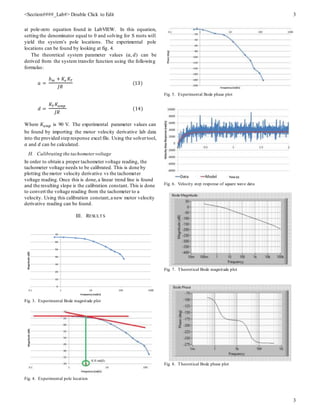
D. Bode Magnitude/Phase Diagrams
In order to find both the Bode magnitude/phase diagrams for
the sinusoidal input voltage data, the motor velocity derivative
is plotted versus time at each individual frequency. Using these
plots, the motor velocity derivative minimum/maximu m
magnitudes are found and an average magnitude is found at
each frequency using the following formula:
𝑀𝑜𝑢𝑡 = 0.5 ∗ (𝜔 𝑚𝑎𝑥 − 𝜔 𝑚𝑖𝑛 ) (6)
Also,the tachometer voltage offset is found using the following
formula:
𝑂𝑜𝑢𝑡 = 0.5 ∗ (𝜔 𝑚𝑎𝑥 + 𝜔 𝑚𝑖𝑛 ) (7)
Once these calculations are complete, the same steps must be
performed for the input waveform (command signal). Once this
is complete, the input sinusoid must be scaled to match the
output sinusoid,and then it is shifted by the offset. This data is
then plotted on the same plot as the motor velocity derivative.
The following plot shows this for 1 Hz frequency range:
Fig. 2. Output/scaled and shifted input vs time for 2 Hz frequency
Once all these plots are made for all frequencies, the next step
is to find the time of several corresponding input/output peaks
for all frequencies. The time difference between each
corresponding input/output peakis the systems delay. Once the
delay is found for each frequency, the phase delay (𝜙)(for each
frequency can be found using the following formula:
𝜙 = 𝑑𝑒𝑙𝑎𝑦 ∗ 𝑠𝑖𝑔𝑛𝑎𝑙 𝑓𝑟𝑒𝑞𝑢𝑒𝑛𝑐𝑦 ∗ 360 (8)
Since the voltage input magnitude entered into LabVIEW was
2 V, the Bode magnitude (𝑀 𝐵𝑜𝑑𝑒 ) can be found using the
following formula:
𝑀 𝐵𝑜𝑑𝑒 = 20 ∗ 𝐿𝑜𝑔10 (
𝑀𝑜𝑢𝑡
𝑀𝑖𝑛
) (9)
Now that both the Bode magnitudes and phase delays have been
found, both Bode plots can be made.
E. Velocity step response plot square wave data
In order to find the velocity step response for the square wave
data, students need to download the given excel file on
Canvas. With this excel file, the motor velocity derivative data
found in lab for the first step wave is pasted into this excel file
as well as the time. When this is done, a plot is created over
the existing plot.
F. Calculating parameter constants
In order to find the theoretical transfer function, bode plots
and pole-zero equations in LabVIEW, the parameter constants
must be calculated. 𝑘 𝑇 , 𝐿, 𝑅, can be found on the given motor
data sheet [2]. 𝑏 𝑚 and 𝐽 must be calculated by hand. 𝑏 𝑚 can be
calculated by using the following formula:
𝑏 𝑚 =
𝑇
𝜔
(10)
𝜔 can be found on the motor data sheet. To calculate the
motor torque, the following formula can be used:
𝑇 = 𝐾𝑇 ∗ 𝑖 (11)
Once the torque is calculated, 𝑏 𝑚 can be found. The rotational
inertia can be found by creating the flywheel in SolidWorks.
G. Estimated gain/ pole locations/parameter values for the
system
The theoretical gain for the systemcan be found by using the
following formula:
𝐾𝑉 =
𝐾𝑇
𝑏 𝑚 𝑅 + 𝐾𝑒 𝐾𝑇
(12)
The experimental gain can be found be looking at the
experimental Bode magnitude plot.
The theoretical pole locations of the systemcan be looking

3. <Section####_Lab#> Double Click to Edit 3
3
at pole-zero equation found in LabVIEW. In this equation,
setting the denominator equal to 0 and solving for S roots will
yield the system’s pole locations. The experimental pole
locations can be found by looking at fig. 4.
The theoretical system parameter values (𝑎, 𝑑) can be
derived from the system transfer function using the following
formulas:
𝑎 =
𝑏 𝑚 + 𝐾𝑒 𝐾𝑇
𝐽𝑅
(13)
𝑑 =
𝐾𝑇 𝐾𝑎𝑚𝑝
𝐽𝑅
(14)
Where 𝐾𝑎𝑚𝑝 is 90 V. The experimental parameter values can
be found by importing the motor velocity derivative lab data
into the provided step response excel file. Using the solvertool,
𝑎 and 𝑑 can be calculated.
H. Calibrating the tachometervoltage
In order to obtain a proper tachometer voltage reading, the
tachometer voltage needs to be calibrated. This is done by
plotting the motor velocity derivative vs the tachometer
voltage reading. Once this is done,a linear trend line is found
and the resulting slope is the calibration constant. This is done
to convert the voltage reading from the tachometer to a
velocity. Using this calibration constant,a new motor velocity
derivative reading can be found.
III. RESULTS
Fig. 3. Experimental Bode magnitude plot
Fig. 4. Experimental pole location
Fig. 5. Experimental Bode phase plot
Fig. 6. Velocity step response of square wave data
Fig. 7. Theoretical Bode magnitude plot
Fig. 8. Theoretical Bode phase plot

4. <Section####_Lab#> Double Click to Edit 4
4
Fig. 9. Theoretical transfer function found in LabVIEW
Fig. 10. Theoretical pole-zero equation found in LabVIEW
Fig. 11. Motor velocity derivative vs time for square waveform plot
Fig. 12. Calibratedmotor velocitytachometer vs timefor square waveformplot
Fig. 13. Motor velocity tachometer vs motor velocity derivative with linear
trendline
TABLE I
THEORETICAL PARAMETER VALUES
Parameter Value
𝐾𝑇 [(N-m)/A] 0.4202
𝐾𝑒 [V/(rad-s)] 0.4202
J [N-m^(2)] 0.0064
R [Ohms] 11
L [H] 0.00028
𝑏 𝑚 [(N-m)/(rad/s)] 0.003157
TABLE II
A AND D PARAMTER VALUES
Parameter Theoretical Experimental
𝑎 2.97 10.31
𝑑 (rad/s) 9.35 6.79
Gain 1.99 1.33
TABLE III
THEORETICAL/EXPERIMENTAL POLE LOCATIONS
Parameter Theoretical Experimental
𝑆1 0 0
𝑆2 -3.00154 4.4
𝑆3 -39,283.2 -
IV. DISCUSSION
A. Comparison of experimental/theoretical Bode plots
Both Bode magnitude plots (figures 3 & 7) have the same
general trend and shape. The main difference is the magnitude
values at which the plots begin/end. The same is true for the
Bode phase plots (figures 5 & 8). The reason for this could be
due to the additional gain constant on the experimental transfer
function.
B. Numerical time derivative vs tachometer voltage
Using the tachometer voltage yields a better reading then the
motor time derivative. This is because the numerical derivative
is a calculated value in LabVIEW which is based on a position
reading. Since a series of calculations has to be performed to
get a motor derivative value, it is more prone to error
propagation. The tachometer voltage is based on a sensor
reading with no intermediate calculations, thus providing a
more accurate reading.
C. Parameter comparison
A 71% difference was calculated between the theoretical 𝑎
value and the experimental 𝑎 value while a 27% error was
calculated between the theoretical 𝑑 value and the
experimental 𝑑 value. These errors are likely due to estimation
errors and noise during data collection.
D. Model improvements
In order to make this model better, closed-loop control could
be used instead of open-loop. This will help account for
numerical errors in the systemby accounting for the system
error in the input command signal. This will help reduce
overshoot and steady-state errors in the system.

5. <Section####_Lab#> Double Click to Edit 5
5
V. CONCLUSION
This lab is a good demonstration of a basic control system.
Using the hardware in lab, an experimental systemmodel was
created to compare to a theoretical system model. This lab
demonstrated that using a motor velocity derivative doesn’t
work as well as using a tachometer voltage reading due to
intermediate calculation errors that propagate. Also, closed-
loop control should be used to account for calculation errors in
LabVIEW.
REFERENCES
[1] N. Instruments, "ModelingDC motorposition,"2008. [Online].
Available: http://www.ni.com/tutorial/6859/en/#toc1.Accessed: Sep. 11,
2016.
[2] Bodine Electric Company, 33ASeries Permanent Magnet DC Motor:
Model 6435specifications. http://www.bodine-
electric.com/Products/Asp/ProductSpecs.asp?Co%E2%80%A6&Name=
33A%20Series%20Permanent%20Magnet%20DC%20Motor&Model=6
[3] S. Banks. “Simplified MF model, EML4312C