Hh3312761282

Nguyen Thanh Phuong, Ho Dac Loc, Tran Quang Thuan / International Journal of Engineering
Research and Applications (IJERA) ISSN: 2248-9622 www.ijera.com
Vol. 3, Issue 3, May-Jun 2013, pp.1276-1282
1276 | P a g e
Control of Two Wheeled Inverted Pendulum Using Silding Mode
Technique
Nguyen Thanh Phuong, Ho Dac Loc, Tran Quang Thuan
Ho Chi Minh City University of Technology (HUTECH) Vietnam
Abstract
In this paper, a controller via sliding
mode control is applied to a two-wheeled inverted
pendulum, which is an inverted pendulum on a
mobile cart carrying two coaxial wheels. The
controller is developed based upon a class of
nonlinear systems whose nonlinear part of the
modeling can be linearly parameterized. The
tracking errors are defined, then the sliding
surface is chosen in an explicit form using
Ackermann’s formula to guarantee that the
tracking error converge to zero asymptotically.
The control law is extracted from the reachability
condition of the sliding surface. In addition, the
overall control system is developed. The
simulation and experimental results on a two-
wheel mobile inverted pendulum are provided to
show the effectiveness of the proposed controller.
Key-Words: - Sliding mode controller, two
wheeled inverted pendulum.
1 Introduction
The two-wheeled inverted pendulum is a
novel type of inverted pendulum. In 2000, Felix
Grasser et al. [1] built successfully a mobile inverted
pendulum JOE. SEGWAY HT was invented by
Dean Kamen in 2001 and made commercially
available in 2003. The basic concept was actually
introduced by Prof. Kazuo Yamafuzi in 1986.
In practice, various inverted pendulum systems
have been developed. Inverted pendulum systems
always exhibit many problems in industrial
applications, for example, nonlinear behaviors under
different operation conditions, external disturbances
and physical constraints on some variables.
Therefore, the task of real time control of an unstable
inverted pendulum is a challenge for the modern
control field.
Chen et al. [2] proposed robust adaptive
control architecture for operation of an inverted
pendulum. Though the stability of the control
strategies can be guaranteed, some prior knowledge
and constraints were required to ensure the stability
of the overall system. Huang et al. [3] proposed a
grey prediction model combined with a PD controller
to balance an inverted pendulum. The control
objective is to swing up the pendulum from a stable
position to an unstable position and to bring its slider
back to the origin of the moving base. However, the
stability of this control scheme cannot be assured.
On the other hand, there are many
literatures on sliding mode control theory, which is
one of the effective nonlinear robust control
approaches. Juergen et al. [4] designed a sliding
mode controller based on Ackermann’s Formula.
Their simulation results prove that the mobile
inverted pendulum can be balanced by this controller.
There is no tracking controller. So tracking controller
of mobile inverted pendulum is deeply needed.
In this paper, a practical controller via
sliding mode control is applied to control two-
wheeled mobile inverted pendulum. The sliding
surface is chosen in an explicit form using
Ackermann’s formula, and the control law is
extracted from the reachability condition of the
sliding surface [5]. Finally, the simulation and
experimental results on computer are presented to
show the effectiveness of the proposed controller.
The two-wheeled mobile inverted pendulum
prototype is shown in Fig. 1. It is composed of a cart
carrying a DC motor coupled to a planetary gearbox
for each wheel, the microcontroller used to
implement the controller, the incremental encoder
and tilt sensor to measure the states, as well as a
vertical pendulum carrying a weight.
Fig. 1 Two-wheeled mobile inverted pendulum
2 System Modelling
In this paper, it is assumed that the wheels
always stay in contact with the ground and that there
will be no slip at the wheel’s contact patches.
The motor dynamics have been considered
[5]. Fig. 2 shows the conversion of the electrical
energy from the DC power supply into the
mechanical energy supplied to the load.

1277 | P a g e
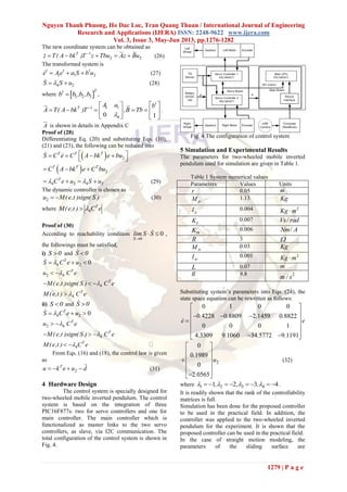
Fig. 2 The diagram of DC motor
The motor model is given as follows [6],
m m e
m
K K K
T V
R R
  (1)
Parameters are given in Appendix A.
Straight Motion Modeling
In straight motion modeling of mobile inverted
pendulum, the left and right wheels are driven under
identical velocity, i.e., rRl xxx   .
The modeling can be linearized by
assuming  , where  represents a small angle
from the vertical direction,
2
1 0
d
cos ,sin ,
dt

  
 
   
 
(2)
The dynamics equation in the straight motion is
as follows [6],
x Ax bu  (3)
22 23 2
42 43 4
0 1 0 0 0
0 0
0 0 0 1 0
0 0
r
r
x
a a bx
A ,x ,b ,
a a b


    
    
      
    
    
    
where 22 23 42 43 2 4a ,a ,a ,a ,b ,b and d are defined as a
function of the system’s parameters, which are given
in Appendix B.
Tracking error is defined as
1
2
3
4
r d
r d
d
d
e x x ,
e x x ,
e ,
e
 
 
 
 
 
 
(4)
where dx is desired value, d is desired inverted
pendulum angle.
Fig. 3 Free body of motion modeling
From Eq. (4), the followings are obtained.
1
2 1
2
3
4 3
4
r d
r d d
r d
d
d d
d
x x e
x x e x e
x x e
e
e e
e
 
  
 
 
   
 
 
   
 
(5)
From Eq. (5), the following can be obtained
2 1
4 3
e e
e e


(6)
Substituting Eq. (5) into Eq. (3), the following can be
obtained.
1 1
2 2
3 3
4 4
d d
d d
d d
d d
x e x e
x e x e
A bu
e e
e e
 
 
    
        
    
   
    
(7)
Rearranging Eq. (7), the following can be obtained
1 1
2 2
3 3
4 4
d d
d d
d d
d d
x xe e
x xe e
A bu A
e e
e e
 
 
      
      
         
      
      
       
(8)
where
rx

1278 | P a g e
22 23
42 43
22 23 2
42 43 4
0 0
0 0
d d d d
d d d d d
d d d d
d d d d d
d d d
d d d
x x x x
x x a x a x
A
a x a
a x a x d
a x a d

   
   

 
       
                
       
       
       
   
        
   
   
    
From Eq. (8), the following error dynamic equation
of mobile inverted pendulum is obtained:
e Ae bu d   (9)
where
1
2 2 2
3
4 4 4
0 0
0 0
e
e b d
e ,b ,d
e
e b d
     
     
       
     
     
     
.
Rearranging Eq. (9), the following can be obtained
  1e Ae b u d Ae bu     (10)
where 1u u d  .
Proof of Eq. (10)
bd d (11)
Because b is not square matrix, the following is
obtained by pseudo inverse of b
 
1
T T
d b b b d

 for 0bbT
 (12)
where   2 2 2
2 4 2 4
4
0
0 0
0
T b
b b b b b b
b
 
 
   
 
 
 
.
If 2 0b  and  4 0 0b b  , Eq. (10) is given as
e Ae (13)
If
2 2
2 4 0b b  ,
 
1
2 2 4 4
2 2
2 4
T T b d b d
d b b b d
b b
 
 

(14)
In this paper,
2 2
2 4 0b b  , dx and d are consider as
constant, so
2 23 4 43
2 2 4 4
d
b a b a
d
b b b b



  
(15)
where d is constant, so d is also constant.
3 Controller Design
The control law u is defined as
1 2au u d u u    (16)
where static controller au contributes the design of
sliding surface, and dynamic controller 2u directly
makes sliding surface attractive to the system state.
The static system is nominal system as follows:
ae Ae bu  (17)
The static controller is given by Ackermann’s
formula as follows:
T
au k e  (18)
 
12 3
0 0 0 1T T T
k h P( A),h , , , b,Ab,A b,A b

     ,
1 2 3 4P( ) ( )( )( )( )            
where 1 2 3 4, , ,    are the desired eigenvalues and
P( ) is characteristic polynomial of Eq. (17).
Substituting Eq. (18) into Eq. (17), the equation of
closed loop system is obtained as
 T
e A bk e  (19)
The sliding surface is chosen as
T T T
1S C e,C h P ( A)  (20)
where 1 1 2 3P( ) ( )( )( )          ,
2 3
1 2 3p p p      .
Proof of Eq. (20)
The left eigenvector T
C of T
A bk associated with
4 satisfies
4
T T T
C ( A bk ) C   (21)
Rearranging Eq. (21) can be obtained as
4
T T T
C ( A I ) C bk  (22)
1 2 3
T T
C b h ( A I )( A I )( A I )b      (23)
 
 
12 3
2 3
1 2 3
0 0 0 1
1
1
T
, , , b,Ab,A b,A b
b Ab A b A b p p p

   
  

Substituting Eqs. (18), (20) and (23) into Eq. (22)
yields
4 1 4
T T T
k C ( A I ) h P( A)( A I )    
T T
k h P( A)
Substituting Eqs. (16) and (18) into Eq. (10), the
dynamic controller as perturbed system is obtained
as follows:
2
T
e ( A bk )e bu   (24)
A new variable z is defined as
1
0
T
e I
z e Te
S C
   
   
     
   
  
(25)
where  1
1 2 3
T
e e ,e ,e is the first three error
variables of e and
T
S C e becomes the last state
variable of z .

1279 | P a g e
The new coordinate system can be obtained as
1
2 2
T
z T( A bk )T z Tbu Az Bu
     (26)
The transformed system is
1 1 1
1 1 2e A e a S b u   (27)
4 2S S u  (28)
where  1
1 2 3
T
b b ,b ,b ,
1
1 11
40 1
T A a b
A T( A bk )T ,B Tb

   
       
   
.
A is shown in details in Appendix C
Proof of (28)
Differentiating Eq. (20) and substituting Eqs. (10),
(21) and (23), the following can be reduced into
  2
T T T
S C e C A bk e bu    
 
  2
T T T
C A bk e C bu  
4 2 4 2
T
C e u S u     (29)
The dynamic controller is chosen as
2u M(e,t )sign( S )  (30)
where 4
T
M(e,t ) C e .
Proof of (30)
According to reachability condition
0
0
S
lim S S

  ,
the followings must be satisfied,
i) S 0 and S 0
4 2 0T
S C e u  
2 4
T
u C e 
4
T
M(e,t )sign( S ) C e  
4
T
M( e,t ) C e
ii) S 0 and S 0
4 2 0T
S C e u  
2 4
T
u C e 
4
T
M(e,t )sign( S ) C e  
4
T
M(e,t ) C e 
From Eqs. (16) and (18), the control law is given
as
2
T
u k e u d    (31)
4 Hardware Design
The control system is specially designed for
two-wheeled mobile inverted pendulum. The control
system is based on the integration of three
PIC16F877s: two for servo controllers and one for
main controller. The main controller which is
functionalized as master links to the two servo
controllers, as slave, via I2C communication. The
total configuration of the control system is shown in
Fig. 4.
Fig. 4 The configuration of control system
5 Simulation and Experimental Results
The parameters for two-wheeled mobile inverted
pendulum used for simulation are given in Table 1.
Table 1 System numerical values
Parameters Values Units
r 0.05 m
pM 1.13 Kg
pI 0.004 2
Kg m
eK 0.007 /Vs rad
mK 0.006 /Nm A
R 3 
wM 0.03 Kg
wI 0.001 2
Kg m
L 0.07 m
g 9.8 2
m / s
Substituting system’s parameters into Eqs. (24), the
state space equation can be rewritten as follows:
0 1 0 0
0 4228 0 8809 2 1459 0 8822
0 0 0 1
4 3309 9 1060 34 5772 9 1191
. . . .
e e
. . . .
 
    
 
 
  
2
0
0 1989
0
2 0565
.
u
.
 
 
 
 
 
 
(32)
where 1 2 3 41 2 3 4, , ,           .
It is readily shown that the rank of the controllability
matrices is full.
Simulation has been done for the proposed controller
to be used in the practical field. In addition, the
controller was applied to the two-wheeled inverted
pendulum for the experiment. It is shown that the
proposed controller can be used in the practical field.
In the case of straight motion modeling, the
parameters of the sliding surface are

1280 | P a g e
1 1   , 2 32 3,     ; the parameters of the
control law is 0 40M  ; the initial values rx , are
zero, and initial errors are 1 1 0e . m  and
3 0 1e . rad  .
Fig. 5 shows that the cart position error has the
convergent time of 5 seconds. Fig. 6 shows that the
inverted pendulum angle error is bounded around
zero after 4 seconds. Fig. 7 shows the sliding surface
to converge zero very fast in simulation.
0 5 10 15
-1
-0.8
-0.6
-0.4
-0.2
0
0.2
0.4
Time(s)
CartPositionError
Cart Position Error(m)
Fig. 5 Cart position error 1 1 0e . m 
0 5 10 15 20 25 30
-0.15
-0.1
-0.05
0
0.05
Time(s)
InvertedPendulumAngleError
Inverted Pendulum Angle Error(rad)
Fig. 6 Inverted pendulum angle error
3 0 1e . rad 
0 2 4 6 8 10
-0.25
-0.2
-0.15
-0.1
-0.05
0
0.05
0.1
Time(s)
SlidingSurface
Fig.7 Sliding surface
Fig. 8 shows controller 1u versus time. Fig. 9 shows
controller 2u versus time. Fig. 10 presents control
law u of mobile inverted pendulum to track
reference.
0 2 4 6 8 10
-40
-30
-20
-10
0
10
20
30
40
50
Time(s)
Input Fig. 8 Dynamic controller 1u
0 2 4 6 8 10
-40
-30
-20
-10
0
10
20
30
40
Time(s)
Input
Fig. 9 Dynamic controller 2u
The experimental results in stable condition are
given after errors converge through Figs.(11) ~ (13).
The encoder voltage is shown in Fig. 11. Fig. 12
presents the output voltage of tilt sensor. Fig. 13
presents motor PWM output under the proposed
controller u in experiment.
0 1 2 3 4 5 6 7 8 9 10
-40
-30
-20
-10
0
10
20
30
40
50
60
Time(s)
ControlInputu
Fig. 10 Controller input u

1281 | P a g e
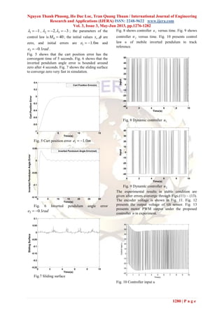
Fig. 11 Output voltage of motor encoder
Fig. 12 Output voltage of tilt sensor
Fig. 13 PWM output of DC motor under control
law
6 Conclusion
This paper presents a sliding mode tracking
controller for the mobile inverted pendulum. The
controller is developed based upon a class of
nonlinear systems whose nonlinear part of the
modeling can be linearly parameterized. The tracking
errors are defined, and then the sliding surface is
chosen in an explicit form using Ackermann’s
formula to guarantee that the tracking error converge
to zero asymptotically.
The simulation and experimental results show
that the proposed controller is applicable and
implemented in the practical field.
REFERENCES:
[1] F. Grasser, A. D’Arrigo, S. Colombi and A.
C. Rufer, JOE: a Mobile, Inverted
Pendulum, IEEE Trans. Industrial
Electronics, Vol. 49, No. 1(2002), pp.
107~114.
[2] C.S. Chen and W.L. Chen: Robust Adaptive
Sliding-mode Control Using Fuzzy
Modeling for an Inverted-pendulum
System, IEEE Trans. Industrial Electronics,
Vol. 45, No. 2(1998), pp. 297~306.
[3] S.J. Huang and C.L. Huang: Control of an
Inverted Pendulum Using Grey Prediction
Model, IEEE Trans. Industrial Applications,
Vol. 36, No. 2(2000), pp. 452~458.
[4] J. Ackermann and V. Utkin: Sliding Mode
Control Design Based on Ackermann’s
Formula, IEEE Trans. Automatic Control,
Vol. 43, No. 2(1998), pp. 234~237.
[5] D. Necsulescu: Mechatronics, Prentice-Hall,
Inc. (2002), pp. 57~60.
[6] M.T. Kang: M.S. Thesis, Control for
Mobile Inverted Pendulum Using Sliding
Mode Technique, Pukyong National
University, (2007).
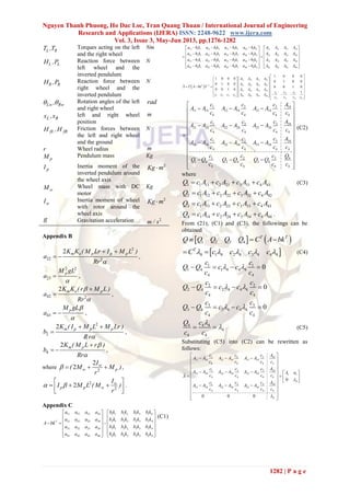
Appendix A
Nomenclature
Variable Description Units
V Motor voltage V
i Current armature A
 Rotor angular velocity rad/s
eV Back electromotive force
voltage
V
eK Back electromotive
voltage coefficient
Vs/rad
RI Inertia moment of the
rotor
2
Kg m
mT Magnetic torque of the
rotor
Nm
mK Magnetic torque
coefficient
Nm/A
T Load torque of the motor Nm
fK Viscous frictional
coefficient of rotor shaft
Nms/ rad
R Nominal rotor resistance 
H Nominal rotor inductance H
cx Cart position
perpendicular to the
wheel axis
m
 Inverted pendulum angle rad
d Desired inverted
pendulum angle
rad
L Distance between the
wheel axis and the
pendulum’s center
m
D Lateral distance between
two coaxial wheels
m

1282 | P a g e
L RT ,T Torques acting on the left
and the right wheel
Nm
L LH ,P Reaction force between
left wheel and the
inverted pendulum
N
R RH ,P Reaction force between
right wheel and the
inverted pendulum
N
Lw Rw,  Rotation angles of the left
and right wheel
rad
L Rx ,x left and right wheel
position
m
fL fRH ,H Friction forces between
the left and right wheel
and the ground
N
r Wheel radius m
pM Pendulum mass Kg
pI Inertia moment of the
inverted pendulum around
the wheel axis
2
Kg m
wM Wheel mass with DC
motor
Kg
wI Inertia moment of wheel
with rotor around the
wheel axis
2
Kg m
g Gravitation acceleration 2
m / s
Appendix B
2
22 2
2 m e p p pK K ( M Lr I M L )
a
Rr 
 
  ,
2 2
23
pM gL
a

 ,
42 2
2 m e pK K ( r M L )
a
Rr



 ,
43
pM gL
a


  ,
2
2
2 m p p pK ( I M L M Lr )
b
Rr
 
 ,
4
2 m pK ( M L r )
b
Rr



  ,
where 2
2
2 w
w p
I
( M M )
r
    ,
2
2
2 w
p p w
I
I M L ( M )
r
 
 
   
 
.
Appendix C
11 12 13 14 1 1 1 2 1 3 1 4
21 22 23 24 2 1 2 2 2 3 2 4
31 32 33 34 3 1 3 2 3 3 3 4
41 42 43 44 4 1 4 2 4 3 4 4
T
a a a a b k b k b k b k
A bk
   
   
     
   
   
   
(C1)
11 1 1 12 1 2 13 1 3 14 1 4 11 12 13 14
21 2 1 22 2 2 23 2 3 24 2 4 21 22 23 24
31 3 1 32 3 2 33 3 3 34 3 4 31 32 33 34
41 4 1 42 4 2 43 4 3 44 4 4 41 42 43 44
a b k a b k a b k a b k A A A A
      
          
     
  
      


 
11 12 13 14
21 22 23 241
31 32 33 34
31 2
1 2 3 4 41 42 43 44
4 4 4 4
1 0 0 0
1 0 0 0
0 1 0 0
0 1 0 0
0 0 1 0
0 0 1 0
1
T
A A A A
A A A A
A T A bk T
A A A A
cc c
c c c c A A A A
c c c c

 
     
     
       
     
             
31 2 14
11 14 12 14 13 14
4 4 4 4
31 2 24
21 24 22 24 23 24
4 4 4 4
3 341 2
31 34 32 34 33 34
4 4 4 4
31 2 4
1 4 2 4 3 4
4 4 4 4
cc c A
A A A A A A
c c c c
cc c A
A A A A A A
c c c c
c Ac c
A A A A A A
c c c c
cc c Q
Q Q Q Q Q Q
c c c c
 
   
 
 
   
 
 
   
 
 
   
  
(C2)
where
1 1 11 2 21 3 31 4 41Q c A c A c A c A    (C3)
2 1 12 2 22 3 32 4 42Q c A c A c A c A   
3 1 13 2 23 3 33 4 43Q c A c A c A c A   
4 1 14 2 24 3 34 4 44Q c A c A c A c A    .
From (21), (C1) and (C3), the followings can be
obtained
   1 2 3 4
T T
Q Q Q Q Q C A bk  
 4 1 4 2 4 3 4 4 4
T
C c c c c      (C4)
1 1
1 4 1 4 4 4
4 4
0
c c
Q Q c c
c c
    
2 2
2 4 2 4 4 4
4 4
0
c c
Q Q c c
c c
    
3 3
3 4 3 4 4 4
4 4
0
c c
Q Q c c
c c
    
4 4 4
4
4 4
Q c
c c

  (C5)
Substituting (C5) into (C2) can be rewritten as
follows:
31 2 14
11 14 12 14 13 14
4 4 4 4
31 2 24
21 24 22 24 23 24 1 1
4 4 4 4
4
3 341 2
31 34 32 34 33 34
4 4 4 4
4
0
0 0 0
cc c A
A A A A A A
c c c c
cc c A
A A A A A A A a
c c c cA
c Ac c
A A A A A A
c c c c


 
   
 
 
     
    
  
   
 
 
 

Hh3312761282

More Related Content

What's hot

Viewers also liked

Similar to Hh3312761282

Recently uploaded

Hh3312761282