This paper discusses PID controller tuning for double integrator systems with dead time, specifically focusing on a real-time ball and beam system. The authors analyze both simulation and real-time responses, providing mathematical models and stability margins for the control system. Experiments reveal discrepancies between simulation and real-time results, attributed to equipment quality and inaccurate time delay selection.

1. Poster Paper
Proc. of Int. Conf. on Advances in Signal Processing and Communication 2013
PID Controller Design for a Real Time Ball and Beam
System – A Double Integrating Process with Dead
Time
I.Thirunavukkarasu1, Marek Zyla2, V.I.George3and Shanmuga Priya4
1& 4
Associate Professor, Dept. of ICE & Chemical Engg, MIT
3
IAESTE Student, AGH Univ. of Science and Tech, Poland.
2
Registrar, Manipal University Jaipur, Rajasthan.
Mail: it.arasu@manipal.edu
Abstract— In this paper, the authors have discussed and shown
how to tune the PID controller in closed loop with time-delay
for the double integrator systems for a particular stability
margins. In math model it is assumed that time delay (ô) of
the plant is known. As a case study the authors have considered the mathematical model of the real-time beam and ball
system and analyzed the simulation and real time response.
or
~
~
K i  ~K p
s
~) 
T (s
~
~ s
~
s
~ 3  ~K e ~  K e ~  ~ 2 K e ~
s
s p s
s
i
d
(2)
where
~  s
s
~
K i  K i m 3
~
K p  K p m 2
Index Terms— double integrator, PID, stability, time delay
I. INTRODUCTION
JWATKINS [1] worked with the PD control for double
integrator systems with time delay. This paper is an extension
in which PID control is analyzed in simulation as well as in
real time. Integral part of the controller eliminates steadystate error, which can be necessary in this kind of systems.
Equations delivered in this paper and m-files based on
them can be helpful in tuning a PID controlled real-time model
of beam and ball system, which is an example of double
integrator system with time delay.
~
K d  K d m
(3)
(4)
(5)
(6)
The characteristic equation of system (2) can be written as
~
~~
~2 ~
s
~ )  1  s K p  s K d  K i e ~
1  L( s
(7)
~3
s
~
~
By setting    magnitude and phase of L ( j  ) in
frequency domain can be written as
II. STABILITY
Consider the feedback control system shown in Fig. 1.
The closed-loop transfer function can be written as
T (s) 
~
L ( j ) 
~
~
~ 2
K 2  K d Ki 
p


~  ~  3 
~
4  


(8)
sK p  K i
3
s
 sK p e  s  K i e  s  s 2 K d e  s
m
~
~ ~
 2 K d  K i  ~
~
 L ( j )  tan 1 
  
~~
 K p



(1)
(9)
Fig. 1. Feedback control system with PID controller and double integrating plant with time delay. It is assumed that velocity (derivative of
controlled value) is known.
© 2013 ACEEE
DOI: 03.LSCS.2013.3.511
96

2. Poster Paper
Proc. of Int. Conf. on Advances in Signal Processing and Communication 2013
~
By setting K d as a parameter, (20) and (21) can be used to
choose gain margin (GM) of the system. The stability
boundary (for gain) can be plotted by setting GM  1 .
Substituting (3), (4), (5), and (6) into (13), (14), (15), (19), (20),
and (21) gives
At gain crossover frequency
~
L ( j
gc )
(10)
 1
~
PM   L ( j  gc )  
(11)
Substituting (9) into (11) gives
0  PM   gc 
~
~ ~
 2 K d  K i  ~
PM  tan 
 
~~
 K p



1
Kp 
(12)
Rearranging (12) it can be shown that
K i (K d ) 

~
0  PM   gc 
2
(22)
 gc
(23)
m  1  tan 2 ( PM   gc )

2
~
 gc K d m   gc 1  cos 2 ( PM   gc )

m
(13)
(24)
Using (8), (10), and (12) it can be shown that
for phase margin plot and
0   pc 
~
 gc
~
Kp 

2
(14)
~
1  tan 2 ( PM   gc )
Kp 


~ ~
~2 ~
~
~
K i ( K d )   gc K d   gc 1  cos 2 ( PM   gc ) (15)
2
 pc
(26)
1  tan 2  pc
mGM
3
 pc
 m

(27)
for gain margin plot.
Combining PM and GM plots for  that satisfy (22) and
(25) stability margins for both phase and gain can be observed
(16)
~
 L ( j  pc )  
(25)
~
2
K
m2 K p
1
 d 
K i (K d )  ~

4
  pc
GM 2
 pc

~
By setting K d as a parameter, (14) and (15) can be used
to choose phase margin of the system. The stability boundary
(as far as phase is concerned) can be plotted by setting
PM  0 .
At the phase crossover frequency
1
~
L ( j  pc )

2
(17)
GM 
for fixed  ,
m , and
K
d
as on Fig. 2 and 3. Fig.
Substituting (9) into (17) gives
~
~2 ~
~  tan 1   pc K d  K i 
 pc
 ~ ~

  pc K p 


(18)
From (18) it can be shown that

~
0   pc 
2
(19)
Using (8), (16), and (18) it can be shown that
~
Kp 
~2
 pc
(20)
~
GM 1  tan 2  pc
~
K
~ ~
K i (K d )   ~ d 

 pc
© 2013 ACEEE
DOI: 03.LSCS.2013.3.511
1
GM
2
~2
Kp
 ~4

pc
Fig. 2. Stability margins of the system. Solid line states for gain and
dashed line for phase. Bold lines are the borders of stability. Below
both bold lines the system is stable. Each step from higher dashed line

 3
~
 pc

to a lower one increases phase margin by
(21)

20 . Each step from
higher solid line to a lower one increases gain margin by
0 .2
highest stability margins are obtained in lower left corner.
97
. The

3. Poster Paper
Proc. of Int. Conf. on Advances in Signal Processing and Communication 2013
Fig. 3. Stability margins of the system. Solid line states for gain and
dashed line for phase. Bold lines are the borders of stability. Below
both bold lines the system is stable. Stability margins are presented as
on Fig. 2
Fig. 5. Step and load disturbance response of the closed-loop system
2 presents plot for   0 .35 , K d  3 and m  0 .7 . Fig.
  0 .1 .
for
3 depicts plot for   0 . 1 , K d  5 and .
parameters:
K
p
T (s) 
III. SIMULATION
 3 .5
,
K i  1 .3
,
0 .7  s
e
s2
Fig. 6. Step response of the real-time system
Fig. 4. Step and load disturbance response of the closed-loop system
parameters:
K
p
 6 .8
,
K i  3 .1 ,
Kd  5,
  0 .1 .
IV. REAL-TIME EXAMPLE
The machine used for real-time experiment was
Googoltech Ball & Beam digital control system. Transfer
function of the model of the system can be written as
© 2013 ACEEE
DOI: 03.LSCS.2013.3.511
(28)
Control was realized by Matlab Simulink, by an already
prepared manufacturer model. The user’s task was only to
put PID gain parameters.
Simulation of the control process was made using Matlab
Simulink software [2-4]. A model was created as on Fig. 1 and
a simulation was run with 2 sets of parameters. Fig. 4 and 5
show step and load disturbance responses of the closedloop system for this two sets of parameters. Load disturbance was a 0.2 step.
for
Kd  5,
Fig. 7. Step response of the real-time system
98

4. Poster Paper
Proc. of Int. Conf. on Advances in Signal Processing and Communication 2013
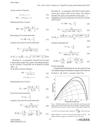
Step responses are shown on Fig. 6 and 7, and load
disturbance response is presented on Fig. 8.
Experiment was made with parameters:
K
p
 6 .8
K i  3 .1
ACKNOWLEDGMENT
The authors thank MIT, Manipal University for providing
the facility for the real time experimentation and the authors
express the gratitude to Dr.Shreesha, Head of the Dept. ICE
and to Mr.Santosh Kumar Chowdhary, In-Charge Space
Engineering Lab, ICE Dept, MIT, Manipal.
(29)
(30)
Kd  5
(31)
It was observed that results of the experiment differ
slightly from ones obtained in the simulation. Overshoot in
the real-time was clearly higher and results were not
repeatable. The main reason is low quality of the equipment.
The ball would become stuck on the beam what made the
model inadequate to reality. Furthermore, the time delay in
simulation was chosen experimentally and it may be
inaccurate.
REFERENCES
[1] J. Watkins, G. Piper, J. Leitner “Control of Time-Delayed
Double Integrator Systems”, Proceedings of the American
Control Conference, Denver, Colorado, 2003, pp. 1506–1511.
[2] Tuyres & Luyben Tuning PI controller for Integral / Time
delayed process, Industrial Engineering chemical research.
Vol.31. P. No: 2625-2628, 1992.
[3] R.Padma Shree and M.Chidambaram “Control of Unstable
System”, Narosa Publications. ISBN: 978-81-7319-700.,2005.
[4] A.Visioli, “Optimal tuning of PID controllers for integral and
unstable processes”, IEE Proc.-Control Theory Appl., Vol. 148,
No. 2. P.No: 180-184, 2001
[5] I.Thirunavukkarasu, “Optimal Robust H ” Controller for an
Integrating Process with Dead Time”, Ph.D Thesis, MIT,
Manipal University, India. 2012.
Fig. 8. Load disturbance response of the real-time system
© 2013 ACEEE
DOI: 03.LSCS.2013.3.511
99