The document discusses the modeling, design, and analysis of a triple inverted pendulum using MATLAB, highlighting the application of optimal control techniques such as linear quadratic regulators (LQR) and pole placement controllers for stabilization. It compares the performance of these controllers, demonstrating that while both can stabilize the system, the pole placement controller offers enhanced stability with less overshoot and shorter settling time than the LQR controller. The findings indicate the effectiveness of feedback control systems in managing the inherently unstable behavior of the inverted pendulum.

1. 1
Comparison of a Triple Inverted Pendulum Stabilization
using Optimal Control Technique
Mustefa Jibril1
, Messay Tadese2
, Eliyas Alemayehu Tadese3
1
Msc, School of Electrical & Computer Engineering, Dire Dawa Institute of Technology, Dire Dawa,
Ethiopia
2
Msc, School of Electrical & Computer Engineering, Dire Dawa Institute of Technology, Dire Dawa,
Ethiopia
3
Msc, Faculty of Electrical & Computer Engineering, Jimma Institute of Technology, Jimma, Ethiopia
Abstract
In this paper, modelling design and analysis of a triple inverted pendulum have been done using
Matlab/Script toolbox. Since a triple inverted pendulum is highly nonlinear, strongly unstable
without using feedback control system. In this paper an optimal control method means a linear
quadratic regulator and pole placement controllers are used to stabilize the triple inverted
pendulum upside. The impulse response simulation of the open loop system shows us that the
pendulum is unstable. The comparison of the closed loop impulse response simulation of the
pendulum with LQR and pole placement controllers results that both controllers have stabilized
the system but the pendulum with LQR controllers have a high overshoot with long settling time
than the pendulum with pole placement controller. Finally the comparison results prove that the
pendulum with pole placement controller improve the stability of the system.
Keywords: Inverted pendulum, linear quadratic regulator, Pole placement.
1. Introduction
An inverted pendulum is a pendulum that has
its center of mass above its pivot point. It is
unstable and without additional assist will
fall over. It may be suspended stably in this
inverted position by means of the usage of a
feedback control system to reveal the angle
of the pole and flow the pivot factor
horizontally returned beneath the center of
mass while it begins to fall over, retaining it
balanced. The inverted pendulum is a classic
problem in dynamics and manage idea and is
used as a benchmark for testing control
techniques. An inverted pendulum is
inherently unstable, and have to be actively
balanced with a view to stay upright; this
could be accomplished either by applying a
torque at the pivot factor, with the aid of
transferring the pivot point horizontally as a
part of a feedback system, changing the state
of rotation of a mass installed at the
pendulum on an axis parallel to the pivot axis
and thereby generating an internal torque at
the pendulum, or with the aid of oscillating
the pivot factor vertically. In order to stabilize
a pendulum in this inverted position, a
feedback control system may be used, which
monitors the pendulum's attitude and actions
the position of the pivot point sideways while
the pendulum starts off evolved to fall over,
to hold it balanced.
2. Mathematical Modeling
The pendulum consists of three arms that are
hinged by ball bearings and can rotate in the
vertical plane. The torques T1 and T2 are the
Preprints (www.preprints.org) | NOT PEER-REVIEWED | Posted: 10 June 2020 doi:10.20944/preprints202006.0128.v1
© 2020 by the author(s). Distributed under a Creative Commons CC BY license.

2. 2
inputs to the pendulum with the middle hinge
made free for rotation. By controlling the
angles of the arms around specified values,
the pendulum can be stabilized inversely with
the desired angle attitudes. The triple inverted
pendulum is shown in Figure 1 below.
Figure 1 the triple pendulum
Let Θi denote the angle of the ith arm
measured from the vertical axis as shown in
Figure 2 below.
Figure 2 System Configuration
The mathematical modelling of the triple
inverted pendulum is derived under the
assumption that each arm is a rigid body
Lagrange differential equations is the method
used to construct the triple pendulum with a
nonlinear vector-matrix differential equation
of the form:
   1
1,2,3
1,2
i i i jM N q GT
i
j
    


Where
 
   
   
   
 
1 1 2 1 2 1 3 1 3
1 2 1 2 2 2 3 2 3
1 3 1 3 2 3 2 3 3
cos cos
cos cos 2
cos cos
J l M l M
M l M J l M
l M l M J
   
    
   
  
 
   
   
Where
1 1 1 2 1 3 1
2 2 2 3 2
3 3 3
M m h m l m l
M m h m l
M m h
  
 

and
2 2 2
1 1 1 1 2 1 3 1
2 2
2 2 2 2 3 2
2
3 3 3 3
J I m h m l m l
J I m h m l
J I m h
   
  
 
The N matrix become:
 
1 2 2
2 2 3 3
3 3
0
3
0
C C C
N C C C C
C C
  
 
    
  
And the q matrix and G matrix are
     
     
       
2 2
1 1 2 1 2 2 1 3 1 3 3 1 1
2 2
2 1 2 1 2 1 2 3 2 3 3 2 2
2 2
3 1 3 1 3 1 1 3 2 3 2 3 2 2 3 3 3
sin sin sin
sin sin sin
sin 2 sin 2 sin
q l M l M M g
q l M l M M g
q l M l M M g
      
      
          
    
    
      
1 0
1 1
0 1
G
 
 
  
  
The description of the system is shown in
Table 1 below
No Symbol Description
1 il length of the ith arm
2 ih the distance from the
bottom to the centre of
gravity
of the ith arm
3 im mass of the ith arm
4 i angle of the ith arm from
vertical line
Preprints (www.preprints.org) | NOT PEER-REVIEWED | Posted: 10 June 2020 doi:10.20944/preprints202006.0128.v1

3. 3
5 iC coefficient of viscous
friction of the ith hinge
6 iI moment of inertia of the
i-th arm around the
centre of
gravity
7 jT control torque of the jth
hinge
After linearization of Equation (2) under the
assumptions of small deviations of the
pendulum from the vertical position and of
small velocities, one obtains the following
equation
 4
1,2,3
1,2
ji i i mM N P GT
i
j
    


Where
 
1 1 2 1 3
1 2 2 2 3
1 3 2 3 3
5
J l M l M
M l M J l M
l M l M J
 
 
  
 
 
And
 
1
2
3
0 0
0 0 6
0 0
M g
P M g
M g
 
 
  
  
The block-diagram of the pendulum system
is shown in Figure 3 and the nominal values
of the parameters are given in Table 2.
Figure 3 Block-diagram of the pendulum
system
Table 2 Nominal values of the parameters
No Symbol Value
1 1h 0.45m
2 2h 0.2m
3 3h 0.3m
4 1l 0.5m
5 2l 0.4m
6 1m 3.5Kg
7 2m 2Kg
8 3m 2.25Kg
9 1I 2
0.55Kg m
10 2I 2
0.12Kg m
11 3I 2
0.65Kg m
12 1C 0.07 N ms
13 2C 0.03N ms
14 3C 0.009 N ms
The state space representation of the triple
inverted pendulum becomes
1
2
3
1
2
3
57.75 14.42 15.82 16.26 5.5 7
25.3 43 12.7 11 13.6 5
178 88.6 55.6 57.3 30.2 25
22.9 10 0.14 0.08 0.04 0.008
26 37.5 3.6 0.15 0.13 0.033
0.83 8.2 9.25 0.01 0.04 0.02






       
  
       
  
 
    
    
 
      
1
2
3 1
1 2
2
3
1
2
3
1
2
3
1.559 0.8
4 3.8
0.65 2.4
0 0
0 0
0 0
1 0 0 0 0 0
0 1 0 0 0 0
0 0 1 0 0 0
0 0 0 1 0 0
0 0 0 0 1 0
0 0 0 0 0 1
T
T
y












   
   
   
     
     
     
    
        
   
  
  
  
  
   
  
  
  
  

3. The Proposed Controllers Design
3.1 LQR Controller Design
The principle of most reliable optimal control
is involved with working a dynamic system
at minimum cost. The case wherein the
system dynamics are described via a fixed of
linear differential equations and the cost is
defined through a quadratic function is
referred to as the LQ problem. One of the
primary outcomes within the theory is that
the solution is furnished with the aid of the
linear quadratic regulator (LQR). The block
diagram of the triple inverted pendulum with
LQR controller is shown below in Figure 4.
Preprints (www.preprints.org) | NOT PEER-REVIEWED | Posted: 10 June 2020 doi:10.20944/preprints202006.0128.v1

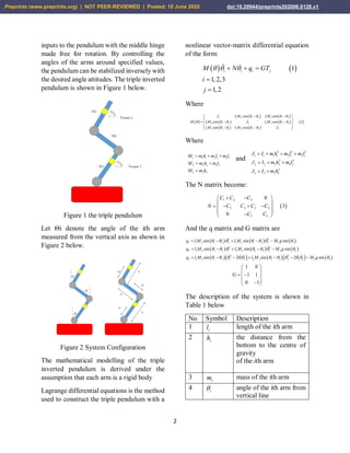
4. 4
Figure 4 Block diagram of the triple inverted
pendulum with LQR controller
In this paper, the value of Q and R is chosen
as
1 0 0 0 0 0
0 1 0 0 0 0
0 0 1 0 0 0 5 0
10
0 0 0 1 0 0 0 5
0 0 0 0 1 0
0 0 0 0 0 1
Q and R
 
 
 
   
    
  
 
  
 
The value of obtained feedback gain matrix
K of LQR is given by
87.4053 32.8355 25.6454 27.1508 11.2981 11.1817
97.7657 45.7910 30.0834 31.2118 15.6479 12.9896
K
 
  
 
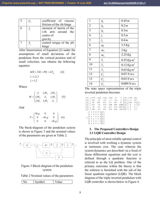
3.2 Pole Placement Controller Design
Pole placement, is a way employed in
feedback control system principle to region
the closed-loop poles of a plant in pre-
decided locations in the s-plane. Placing
poles is proper because the region of the poles
corresponds immediately to the eigenvalues
of the system, which control the traits of the
reaction of the system. The system ought to
be considered controllable on the way to put
into effect this technique. The block diagram
of the triple inverted pendulum with pole
placement controller is shown in Figure 5.
Figure 5 Block diagram of the triple inverted
pendulum with pole placement controller
The state equations for the closed-loop
system of Figure 5 can be written by
inspection as
     7x Ax Bu Ax B Kx A BK x
y Cx
      

The poles for this system is chosen as
 P = 1, 2, 3, 4, 5, 6     
Solving using Matlab the robust pole
placement algorithm gain will be
19329 8885 7472 11601 5861 6699
23483 10820 9086 14362 7268 8307
K
 
  
 
4. Result and Discussion
4.1 Controllability and Observability
of the Pendulum
A system (state space representation) is
controllable iff the controllable matrix C = [B
AB A2B….An-1B] has rank n where n is the
number of degrees of freedom of the system.
In our system, the controllable matrix C = [B
AB A2B A3B A4B A5B] has rank 6 which
the degree of freedom of the system. So, the
system is controllable.
A system (state space representation) is
Observable iff the Observable matrix D = [C
CA CA2….CAn-1] T has a full rank n.
Preprints (www.preprints.org) | NOT PEER-REVIEWED | Posted: 10 June 2020 doi:10.20944/preprints202006.0128.v1

5. 5
In our system, the Observable matrix D = [C
CA CA2 CA3 CA4 CA5] T has a full rank of
6. So, the system is Observable.
4.2 Open Loop Impulse Response of
the Triple Inverted Pendulum
The open loop simulation for a 1 Nm impulse
input of torque 1 for angular displacement 1,
2 and 3 and for angular velocity 1, 2 and 3 is
shown in Figure 6, 7, 8, 9, 10 and 11 and for
torque 2 input the angular displacement 1, 2
and 3 and for angular velocity 1, 2 and 3 is
shown in Figure 12, 13, 14, 15, 16 and 17
respectively.
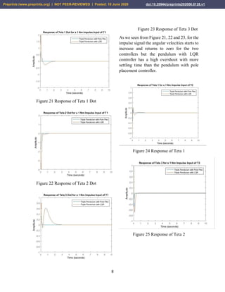
Figure 6 Response of Teta 1
Figure 7 Response of Teta 2
Figure 8 Response of Teta 3
Figure 9 Response of Teta 1 Dot
Figure 10 Response of Teta 2 Dot
Preprints (www.preprints.org) | NOT PEER-REVIEWED | Posted: 10 June 2020 doi:10.20944/preprints202006.0128.v1

6. 6
Figure 11 Response of Teta 3 Dot
Figure 12 Response of Teta 1
Figure 13 Response of Teta 2
Figure 14 Response of Teta 3
Figure 15 Response of Teta 1 Dot
Figure 16 Response of Teta 2 Dot
Preprints (www.preprints.org) | NOT PEER-REVIEWED | Posted: 10 June 2020 doi:10.20944/preprints202006.0128.v1

7. 7
Figure 17 Response of Teta 3 Dot
As we seen from the Figures above the
angular displacements and the angular
velocities are unstable.
4.3 Comparison of the Triple Inverted
Pendulum with LQR and Pole
Placement Controllers for Impulse
Input Signal
The comparison of the triple inverted
pendulum with LQR and pole placement
controller for a 1 Nm impulse input of torque
1 for angular displacement 1, 2 and 3 and for
angular velocity 1, 2 and 3 is shown in Figure
18, 19, 20, 21, 22 and 23 and for torque 2
input the angular displacement 1, 2 and 3 and
for angular velocity 1, 2 and 3 is shown in
Figure 24, 25, 26, 27, 28 and 29 respectively.
Figure 18 Response of Teta 1
Figure 19 Response of Teta 2
Figure 20 Response of Teta 3
As we seen from Figure 18, 19 and 20, for the
impulse signal the angles starts to increase
and returns to zero degree for the two
controllers but the pendulum with LQR
controller has a high overshoot with more
settling time than the pendulum with pole
placement controller.
Preprints (www.preprints.org) | NOT PEER-REVIEWED | Posted: 10 June 2020 doi:10.20944/preprints202006.0128.v1

8. 8
Figure 21 Response of Teta 1 Dot
Figure 22 Response of Teta 2 Dot
Figure 23 Response of Teta 3 Dot
As we seen from Figure 21, 22 and 23, for the
impulse signal the angular velocities starts to
increase and returns to zero for the two
controllers but the pendulum with LQR
controller has a high overshoot with more
settling time than the pendulum with pole
placement controller.
Figure 24 Response of Teta 1
Figure 25 Response of Teta 2
Preprints (www.preprints.org) | NOT PEER-REVIEWED | Posted: 10 June 2020 doi:10.20944/preprints202006.0128.v1

9. 9
Figure 26 Response of Teta 3
As we seen from Figure 24, 25 and 26, for the
impulse signal the angles starts to increase
and returns to zero degree for the two
controllers but the pendulum with LQR
controller has a high overshoot with more
settling time than the pendulum with pole
placement controller.
Figure 27 Response of Teta 1 Dot
Figure 28 Response of Teta 2 Dot
Figure 29 Response of Teta 3 Dot
As we seen from Figure 27, 28 and 29, for the
impulse signal the angular velocities starts to
increase and returns to zero for the two
controllers but the pendulum with LQR
controller has a high overshoot with more
settling time than the pendulum with pole
placement controller.
5. Conclusion
In this paper, stabilization of the triple
inverted pendulum with LQR and pole
placement controller have been analyzed
simulated and compared suceesfully. The
Preprints (www.preprints.org) | NOT PEER-REVIEWED | Posted: 10 June 2020 doi:10.20944/preprints202006.0128.v1

10. 10
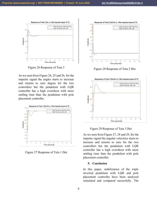
open loop simulation prove that the system is
not stable without feedback control system.
Comparison of the proposed controllers for
an impulse input have been done and the
system with pole placement controller
improves the stability of the system.
Reference
[1].Mustefa Jibril et al. “Robust Control
Theory Based Performance
Investigation of an Inverted
Pendulum System using Simulink”
International Journal of Advance
Research and Innovative Ideas in
Education, Vol. 6, Issue 2, pp. 808-
814, 2020.
[2].Ali Rohan et al. “Design of Fuzzy
Logic Based Controller for
Gyroscopic Inverted Pendulum
System” Int. J. Fuzzy Log. Intell.
Syst, Vol. 18, Issue 1, pp. 58-64,
2018.
[3].Xiaoping H. et al. “Optimization of
Triple Inverted Pendulum Control
Process Based on Motion Vision”
EURASIP Journal on Image and
Video Processing, No. 73, 2018.
[4].R. Dimas P. et al. “Implementation of
Push Recovery Strategy using Triple
Linear Inverted Pendulum Model in
T-Flow Humanoid Robot” Journal of
Physics: Conference Series, Vol.
1007, 2018.
[5].Wei Chen et al. “Simulation of a
Triple Inverted Pendulum Based on
Fuzzy Control” WJET, Vol. 4, No. 2,
2016.
[6].Tang Y et al. “A New Fuzzy
Evidential Controller for
Stabilization of the Planar Inverted
Pendulum System” PLOS ONE, Vol.
11, Issue 8, 2016.
[7].Yuanhong D. et al. “Multi Mode
Control Based on HSIC for Double
Pendulum Robot” Journal of
Vibroengineering, Vol. 17, Issue 7,
pp. 3683-3692, 2015.
Preprints (www.preprints.org) | NOT PEER-REVIEWED | Posted: 10 June 2020 doi:10.20944/preprints202006.0128.v1