Download as PDF, PPTX
![11
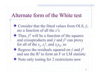
The Breusch-Pagan Test
Don’t observe the error, but can estimate it with
the residuals from the OLS regression
After regressing the residuals squared on all of the
x’s, can use the R2 to form an F or LM test
The F statistic is just the reported F statistic for
overall significance of the regression, F =
[R2/k]/[(1 – R2)/(n – k – 1)], which is distributed
Fk, n – k - 1
The LM statistic is LM = nR2, which is distributed
c2
k](https://image.slidesharecdn.com/ch08-150712112224-lva1-app6891/85/Chapter8-11-320.jpg)

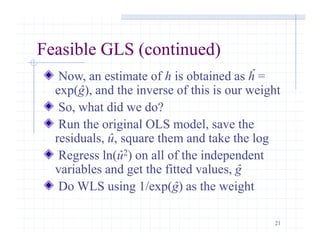
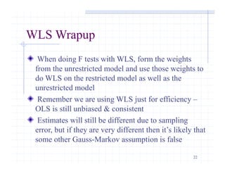

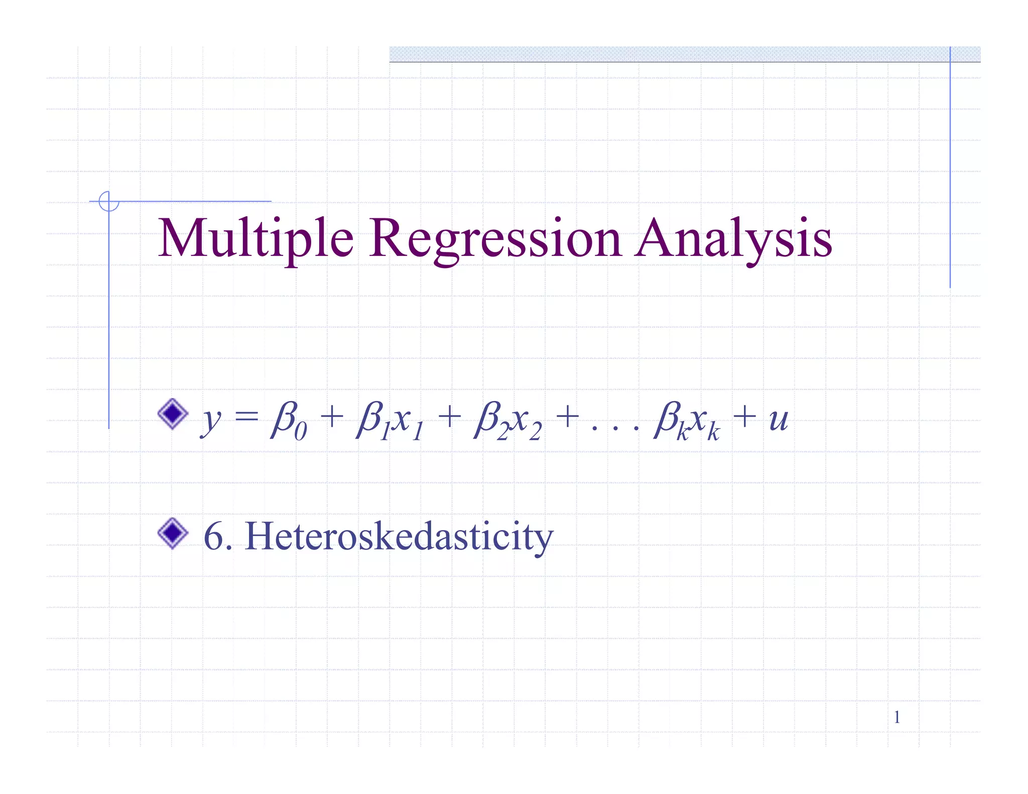
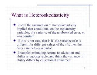
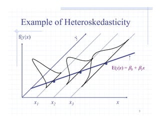
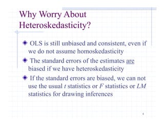
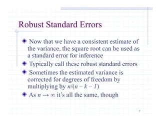
This document discusses heteroskedasticity in multiple linear regression models. Heteroskedasticity occurs when the variance of the error term is not constant, violating the assumption of homoskedasticity. If heteroskedasticity is present, ordinary least squares (OLS) estimates are still unbiased but the standard errors are biased. Various tests for heteroskedasticity are presented, including the Breusch-Pagan and White tests. Weighted least squares (WLS) methods like feasible generalized least squares (FGLS) can produce more efficient estimates than OLS when the form of heteroskedasticity is known or can be estimated.