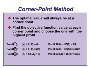
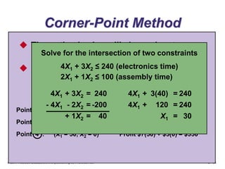
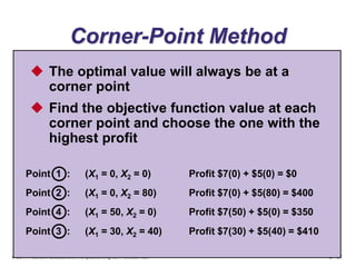
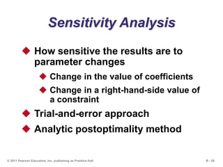
B - 1© 2011 Pearson Education, Inc. publishing as Prentice Hall
B Linear Programming
PowerPoint presentation to accompany
Heizer and Render
Operations Management, 10e
Principles of Operations Management, 8e
PowerPoint slides by Jeff Heyl
B - 2© 2011 Pearson Education, Inc. publishing as Prentice Hall
Outline
 Why Use Linear Programming?
 Requirements of a Linear
Programming Problem
 Formulating Linear Programming
Problems
 Shader Electronics Example
B - 3© 2011 Pearson Education, Inc. publishing as Prentice Hall
Outline – Continued
 Graphical Solution to a Linear
Programming Problem
 Graphical Representation of
Constraints
 Iso-Profit Line Solution Method
 Corner-Point Solution Method
B - 4© 2011 Pearson Education, Inc. publishing as Prentice Hall
Outline – Continued
 Sensitivity Analysis
 Sensitivity Report
 Changes in the Resources of the
Right-Hand-Side Values
 Changes in the Objective Function
Coefficient
 Solving Minimization Problems
B - 5© 2011 Pearson Education, Inc. publishing as Prentice Hall
Outline – Continued
 Linear Programming Applications
 Production-Mix Example
 Diet Problem Example
 Labor Scheduling Example
 The Simplex Method of LP
B - 6© 2011 Pearson Education, Inc. publishing as Prentice Hall
Learning Objectives
When you complete this module you
should be able to:
1. Formulate linear programming
models, including an objective
function and constraints
2. Graphically solve an LP problem with
the iso-profit line method
3. Graphically solve an LP problem with
the corner-point method
B - 7© 2011 Pearson Education, Inc. publishing as Prentice Hall
Learning Objectives
When you complete this module you
should be able to:
4. Interpret sensitivity analysis and
shadow prices
5. Construct and solve a minimization
problem
6. Formulate production-mix, diet, and
labor scheduling problems
B - 8© 2011 Pearson Education, Inc. publishing as Prentice Hall
Why Use Linear Programming?
 A mathematical technique to
help plan and make decisions
relative to the trade-offs
necessary to allocate resources
 Will find the minimum or
maximum value of the objective
 Guarantees the optimal solution
to the model formulated
B - 9© 2011 Pearson Education, Inc. publishing as Prentice Hall
LP Applications
1. Scheduling school buses to minimize
total distance traveled
2. Allocating police patrol units to high
crime areas in order to minimize
response time to 911 calls
3. Scheduling tellers at banks so that
needs are met during each hour of the
day while minimizing the total cost of
labor
B - 10© 2011 Pearson Education, Inc. publishing as Prentice Hall
LP Applications
4. Selecting the product mix in a factory
to make best use of machine- and
labor-hours available while maximizing
the firm’s profit
5. Picking blends of raw materials in feed
mills to produce finished feed
combinations at minimum costs
6. Determining the distribution system
that will minimize total shipping cost
B - 11© 2011 Pearson Education, Inc. publishing as Prentice Hall
LP Applications
7. Developing a production schedule that
will satisfy future demands for a firm’s
product and at the same time minimize
total production and inventory costs
8. Allocating space for a tenant mix in a
new shopping mall
so as to maximize
revenues to the
leasing company
B - 12© 2011 Pearson Education, Inc. publishing as Prentice Hall
Requirements of an
LP Problem
1. LP problems seek to maximize or
minimize some quantity (usually
profit or cost) expressed as an
objective function
2. The presence of restrictions, or
constraints, limits the degree to
which we can pursue our
objective
B - 13© 2011 Pearson Education, Inc. publishing as Prentice Hall
Requirements of an
LP Problem
3. There must be alternative courses
of action to choose from
4. The objective and constraints in
linear programming problems
must be expressed in terms of
linear equations or inequalities
B - 14© 2011 Pearson Education, Inc. publishing as Prentice Hall
Formulating LP Problems
The product-mix problem at Shader Electronics
 Two products
1. Shader x-pod, a portable music
player
2. Shader BlueBerry, an internet-
connected color telephone
 Determine the mix of products that will
produce the maximum profit
B - 15© 2011 Pearson Education, Inc. publishing as Prentice Hall
Formulating LP Problems
x-pods BlueBerrys Available Hours
Department (X1) (X2) This Week
Hours Required
to Produce 1 Unit
Electronic 4 3 240
Assembly 2 1 100
Profit per unit $7 $5
Decision Variables:
X1 = number of x-pods to be produced
X2 = number of BlueBerrys to be produced
Table B.1
B - 16© 2011 Pearson Education, Inc. publishing as Prentice Hall
Formulating LP Problems
Objective Function:
Maximize Profit = $7X1 + $5X2
There are three types of constraints
 Upper limits where the amount used is ≤
the amount of a resource
 Lower limits where the amount used is ≥
the amount of the resource
 Equalities where the amount used is =
the amount of the resource
B - 17© 2011 Pearson Education, Inc. publishing as Prentice Hall
Formulating LP Problems
Second Constraint:
2X1 + 1X2 ≤ 100 (hours of assembly time)
Assembly
time available
Assembly
time used is ≤
First Constraint:
4X1 + 3X2 ≤ 240 (hours of electronic time)
Electronic
time available
Electronic
time used is ≤
B - 18© 2011 Pearson Education, Inc. publishing as Prentice Hall
Graphical Solution
 Can be used when there are two
decision variables
1. Plot the constraint equations at their
limits by converting each equation
to an equality
2. Identify the feasible solution space
3. Create an iso-profit line based on
the objective function
4. Move this line outwards until the
optimal point is identified
B - 19© 2011 Pearson Education, Inc. publishing as Prentice Hall
Graphical Solution
100 –
–
80 –
–
60 –
–
40 –
–
20 –
–
–| | | | | | | | | | |
0 20 40 60 80 100
NumberofBlueBerrys
Number of x-pods
X1
X2
Assembly (Constraint B)
Electronics (Constraint A)
Feasible
region
Figure B.3
B - 20© 2011 Pearson Education, Inc. publishing as Prentice Hall
Graphical Solution
100 –
–
80 –
–
60 –
–
40 –
–
20 –
–
–| | | | | | | | | | |
0 20 40 60 80 100
NumberofBlueBerrys
Number of x-pods
X1
X2
Assembly (Constraint B)
Electronics (Constraint A)
Feasible
region
Figure B.3
Iso-Profit Line Solution Method
Choose a possible value for the
objective function
$210 = 7X1 + 5X2
Solve for the axis intercepts of the function
and plot the line
X2 = 42 X1 = 30
B - 21© 2011 Pearson Education, Inc. publishing as Prentice Hall
Graphical Solution
100 –
–
80 –
–
60 –
–
40 –
–
20 –
–
–| | | | | | | | | | |
0 20 40 60 80 100
NumberofBlueBerrys
Number of x-pods
X1
X2
Figure B.4
(0, 42)
(30, 0)
$210 = $7X1 + $5X2
B - 22© 2011 Pearson Education, Inc. publishing as Prentice Hall
Graphical Solution
100 –
–
80 –
–
60 –
–
40 –
–
20 –
–
–| | | | | | | | | | |
0 20 40 60 80 100
NumberofBlueBerrys
Number of x-pods
X1
X2
Figure B.5
$210 = $7X1 + $5X2
$420 = $7X1 + $5X2
$350 = $7X1 + $5X2
$280 = $7X1 + $5X2
B - 23© 2011 Pearson Education, Inc. publishing as Prentice Hall
Graphical Solution
100 –
–
80 –
–
60 –
–
40 –
–
20 –
–
–| | | | | | | | | | |
0 20 40 60 80 100
NumberofBlueBerrys
Number of x-pods
X1
X2
Figure B.6
$410 = $7X1 + $5X2
Maximum profit line
Optimal solution point
(X1 = 30, X2 = 40)
B - 24© 2011 Pearson Education, Inc. publishing as Prentice Hall
100 –
–
80 –
–
60 –
–
40 –
–
20 –
–
–| | | | | | | | | | |
0 20 40 60 80 100
NumberofBlueBerrys
Number of x-pods
X1
X2
Corner-Point Method
Figure B.7
1
2
3
4
B - 25© 2011 Pearson Education, Inc. publishing as Prentice Hall
Corner-Point Method
 The optimal value will always be at a
corner point
 Find the objective function value at each
corner point and choose the one with the
highest profit
Point 1 : (X1 = 0, X2 = 0) Profit $7(0) + $5(0) = $0
Point 2 : (X1 = 0, X2 = 80) Profit $7(0) + $5(80) = $400
Point 4 : (X1 = 50, X2 = 0) Profit $7(50) + $5(0) = $350
B - 26© 2011 Pearson Education, Inc. publishing as Prentice Hall
Corner-Point Method
 The optimal value will always be at a
corner point
 Find the objective function value at each
corner point and choose the one with the
highest profit
Point 1 : (X1 = 0, X2 = 0) Profit $7(0) + $5(0) = $0
Point 2 : (X1 = 0, X2 = 80) Profit $7(0) + $5(80) = $400
Point 4 : (X1 = 50, X2 = 0) Profit $7(50) + $5(0) = $350
Solve for the intersection of two constraints
2X1 + 1X2 ≤ 100 (assembly time)
4X1 + 3X2 ≤ 240 (electronics time)
4X1 + 3X2 = 240
- 4X1 - 2X2 = -200
+ 1X2 = 40
4X1 + 3(40) = 240
4X1 + 120 = 240
X1 = 30
B - 27© 2011 Pearson Education, Inc. publishing as Prentice Hall
Corner-Point Method
 The optimal value will always be at a
corner point
 Find the objective function value at each
corner point and choose the one with the
highest profit
Point 1 : (X1 = 0, X2 = 0) Profit $7(0) + $5(0) = $0
Point 2 : (X1 = 0, X2 = 80) Profit $7(0) + $5(80) = $400
Point 4 : (X1 = 50, X2 = 0) Profit $7(50) + $5(0) = $350
Point 3 : (X1 = 30, X2 = 40) Profit $7(30) + $5(40) = $410
B - 28© 2011 Pearson Education, Inc. publishing as Prentice Hall
Sensitivity Analysis
 How sensitive the results are to
parameter changes
 Change in the value of coefficients
 Change in a right-hand-side value of
a constraint
 Trial-and-error approach
 Analytic postoptimality method
B - 29© 2011 Pearson Education, Inc. publishing as Prentice Hall
Sensitivity Report
Program B.1
B - 30© 2011 Pearson Education, Inc. publishing as Prentice Hall
Changes in Resources
 The right-hand-side values of
constraint equations may change
as resource availability changes
 The shadow price of a constraint is
the change in the value of the
objective function resulting from a
one-unit change in the right-hand-
side value of the constraint
B - 31© 2011 Pearson Education, Inc. publishing as Prentice Hall
Changes in Resources
 Shadow prices are often explained
as answering the question “How
much would you pay for one
additional unit of a resource?”
 Shadow prices are only valid over a
particular range of changes in right-
hand-side values
 Sensitivity reports provide the
upper and lower limits of this range
B - 32© 2011 Pearson Education, Inc. publishing as Prentice Hall
Sensitivity Analysis
–
100 –
–
80 –
–
60 –
–
40 –
–
20 –
–
–| | | | | | | | | | |
0 20 40 60 80 100 X1
X2
Figure B.8 (a)
Changed assembly constraint from
2X1 + 1X2 = 100
to 2X1 + 1X2 = 110
Electronics constraint
is unchanged
Corner point 3 is still optimal, but
values at this point are now X1 = 45,
X2 = 20, with a profit = $415
1
2
3
4
B - 33© 2011 Pearson Education, Inc. publishing as Prentice Hall
Sensitivity Analysis
–
100 –
–
80 –
–
60 –
–
40 –
–
20 –
–
–| | | | | | | | | | |
0 20 40 60 80 100 X1
X2
Figure B.8 (b)
Changed assembly constraint from
2X1 + 1X2 = 100
to 2X1 + 1X2 = 90
Electronics constraint
is unchanged
Corner point 3 is still optimal, but
values at this point are now X1 = 15,
X2 = 60, with a profit = $405
1
2
3
4
B - 34© 2011 Pearson Education, Inc. publishing as Prentice Hall
Changes in the
Objective Function
 A change in the coefficients in the
objective function may cause a
different corner point to become the
optimal solution
 The sensitivity report shows how
much objective function
coefficients may change without
changing the optimal solution point
B - 35© 2011 Pearson Education, Inc. publishing as Prentice Hall
Solving Minimization
Problems
 Formulated and solved in much the
same way as maximization
problems
 In the graphical approach an iso-
cost line is used
 The objective is to move the iso-
cost line inwards until it reaches
the lowest cost corner point
B - 36© 2011 Pearson Education, Inc. publishing as Prentice Hall
Minimization Example
X1 = number of tons of black-and-white picture
chemical produced
X2 = number of tons of color picture chemical
produced
Minimize total cost = 2,500X1 + 3,000X2
Subject to:
X1 ≥ 30 tons of black-and-white chemical
X2 ≥ 20 tons of color chemical
X1 + X2 ≥ 60 tons total
X1, X2 ≥ $0 nonnegativity requirements
B - 37© 2011 Pearson Education, Inc. publishing as Prentice Hall
Minimization Example
Table B.9
60 –
50 –
40 –
30 –
20 –
10 –
–| | | | | | |
0 10 20 30 40 50 60
X1
X2
Feasible
region
X1 = 30
X2 = 20
X1 + X2 = 60
b
a
B - 38© 2011 Pearson Education, Inc. publishing as Prentice Hall
Minimization Example
Total cost at a = 2,500X1 + 3,000X2
= 2,500 (40) + 3,000(20)
= $160,000
Total cost at b = 2,500X1 + 3,000X2
= 2,500 (30) + 3,000(30)
= $165,000
Lowest total cost is at point a
B - 39© 2011 Pearson Education, Inc. publishing as Prentice Hall
LP Applications
Production-Mix Example
Department
Product Wiring Drilling Assembly Inspection Unit Profit
XJ201 .5 3 2 .5 $ 9
XM897 1.5 1 4 1.0 $12
TR29 1.5 2 1 .5 $15
BR788 1.0 3 2 .5 $11
Capacity Minimum
Department (in hours) Product Production Level
Wiring 1,500 XJ201 150
Drilling 2,350 XM897 100
Assembly 2,600 TR29 300
Inspection 1,200 BR788 400
B - 40© 2011 Pearson Education, Inc. publishing as Prentice Hall
LP Applications
X1 = number of units of XJ201 produced
X2 = number of units of XM897 produced
X3 = number of units of TR29 produced
X4 = number of units of BR788 produced
Maximize profit = 9X1 + 12X2 + 15X3 + 11X4
subject to .5X1 + 1.5X2 + 1.5X3 + 1X4 ≤ 1,500 hours of wiring
3X1 + 1X2 + 2X3 + 3X4 ≤ 2,350 hours of drilling
2X1 + 4X2 + 1X3 + 2X4 ≤ 2,600 hours of assembly
.5X1 + 1X2 + .5X3 + .5X4 ≤ 1,200 hours of inspection
X1 ≥ 150 units of XJ201
X2 ≥ 100 units of XM897
X3 ≥ 300 units of TR29
X4 ≥ 400 units of BR788
B - 41© 2011 Pearson Education, Inc. publishing as Prentice Hall
LP Applications
Diet Problem Example
A 3 oz 2 oz 4 oz
B 2 oz 3 oz 1 oz
C 1 oz 0 oz 2 oz
D 6 oz 8 oz 4 oz
Feed
Product Stock X Stock Y Stock Z
B - 42© 2011 Pearson Education, Inc. publishing as Prentice Hall
LP Applications
X1 = number of pounds of stock X purchased per cow each month
X2 = number of pounds of stock Y purchased per cow each month
X3 = number of pounds of stock Z purchased per cow each month
Minimize cost = .02X1 + .04X2 + .025X3
Ingredient A requirement: 3X1 + 2X2 + 4X3 ≥ 64
Ingredient B requirement: 2X1 + 3X2 + 1X3 ≥ 80
Ingredient C requirement: 1X1 + 0X2 + 2X3 ≥ 16
Ingredient D requirement: 6X1 + 8X2 + 4X3 ≥ 128
Stock Z limitation: X3 ≤ 80
X1, X2, X3 ≥ 0
Cheapest solution is to purchase 40 pounds of grain X
at a cost of $0.80 per cow
B - 43© 2011 Pearson Education, Inc. publishing as Prentice Hall
LP Applications
Labor Scheduling Example
F = Full-time tellers
P1 = Part-time tellers starting at 9 AM (leaving at 1 PM)
P2 = Part-time tellers starting at 10 AM (leaving at 2 PM)
P3 = Part-time tellers starting at 11 AM (leaving at 3 PM)
P4 = Part-time tellers starting at noon (leaving at 4 PM)
P5 = Part-time tellers starting at 1 PM (leaving at 5 PM)
Time Number of Time Number of
Period Tellers Required Period Tellers Required
9 AM - 10 AM 10 1 PM - 2 PM 18
10 AM - 11 AM 12 2 PM - 3 PM 17
11 AM - Noon 14 3 PM - 4 PM 15
Noon - 1 PM 16 4 PM - 5 PM 10
B - 44© 2011 Pearson Education, Inc. publishing as Prentice Hall
LP Applications
= $75F + $24(P1 + P2 + P3 + P4 + P5)
Minimize total daily
manpower cost
F + P1 ≥ 10 (9 AM - 10 AM needs)
F + P1 + P2 ≥ 12 (10 AM - 11 AM needs)
1/2 F + P1 + P2 + P3 ≥ 14 (11 AM - 11 AM needs)
1/2 F + P1 + P2 + P3 + P4 ≥ 16 (noon - 1 PM needs)
F + P2 + P3 + P4 + P5 ≥ 18 (1 PM - 2 PM needs)
F + P3 + P4 + P5 ≥ 17 (2 PM - 3 PM needs)
F + P4 + P5 ≥ 15 (3 PM - 7 PM needs)
F + P5 ≥ 10 (4 PM - 5 PM needs)
F ≤ 12
4(P1 + P2 + P3 + P4 + P5) ≤ .50(10 + 12 + 14 + 16 + 18 + 17 + 15 + 10)
B - 45© 2011 Pearson Education, Inc. publishing as Prentice Hall
LP Applications
= $75F + $24(P1 + P2 + P3 + P4 + P5)
Minimize total daily
manpower cost
F + P1 ≥ 10 (9 AM - 10 AM needs)
F + P1 + P2 ≥ 12 (10 AM - 11 AM needs)
1/2 F + P1 + P2 + P3 ≥ 14 (11 AM - 11 AM needs)
1/2 F + P1 + P2 + P3 + P4 ≥ 16 (noon - 1 PM needs)
F + P2 + P3 + P4 + P5 ≥ 18 (1 PM - 2 PM needs)
F + P3 + P4 + P5 ≥ 17 (2 PM - 3 PM needs)
F + P4 + P5 ≥ 15 (3 PM - 7 PM needs)
F + P5 ≥ 10 (4 PM - 5 PM needs)
F ≤ 12
4(P1 + P2 + P3 + P4 + P5) ≤ .50(112)
F, P1, P2, P3, P4, P5 ≥ 0
B - 46© 2011 Pearson Education, Inc. publishing as Prentice Hall
LP Applications
There are two alternate optimal solutions to this
problem but both will cost $1,086 per day
F = 10 F = 10
P1 = 0 P1 = 6
P2 = 7 P2 = 1
P3 = 2 P3 = 2
P4 = 2 P4 = 2
P5 = 3 P5 = 3
First Second
Solution Solution
B - 47© 2011 Pearson Education, Inc. publishing as Prentice Hall
The Simplex Method
 Real world problems are too
complex to be solved using the
graphical method
 The simplex method is an algorithm
for solving more complex problems
 Developed by George Dantzig in the
late 1940s
 Most computer-based LP packages
use the simplex method
B - 48© 2011 Pearson Education, Inc. publishing as Prentice Hall
All rights reserved. No part of this publication may be reproduced, stored in a retrieval
system, or transmitted, in any form or by any means, electronic, mechanical, photocopying,
recording, or otherwise, without the prior written permission of the publisher.
Printed in the United States of America.

Heizer om10 mod_b

  • 1.
    B - 1©2011 Pearson Education, Inc. publishing as Prentice Hall B Linear Programming PowerPoint presentation to accompany Heizer and Render Operations Management, 10e Principles of Operations Management, 8e PowerPoint slides by Jeff Heyl
  • 2.
    B - 2©2011 Pearson Education, Inc. publishing as Prentice Hall Outline  Why Use Linear Programming?  Requirements of a Linear Programming Problem  Formulating Linear Programming Problems  Shader Electronics Example
  • 3.
    B - 3©2011 Pearson Education, Inc. publishing as Prentice Hall Outline – Continued  Graphical Solution to a Linear Programming Problem  Graphical Representation of Constraints  Iso-Profit Line Solution Method  Corner-Point Solution Method
  • 4.
    B - 4©2011 Pearson Education, Inc. publishing as Prentice Hall Outline – Continued  Sensitivity Analysis  Sensitivity Report  Changes in the Resources of the Right-Hand-Side Values  Changes in the Objective Function Coefficient  Solving Minimization Problems
  • 5.
    B - 5©2011 Pearson Education, Inc. publishing as Prentice Hall Outline – Continued  Linear Programming Applications  Production-Mix Example  Diet Problem Example  Labor Scheduling Example  The Simplex Method of LP
  • 6.
    B - 6©2011 Pearson Education, Inc. publishing as Prentice Hall Learning Objectives When you complete this module you should be able to: 1. Formulate linear programming models, including an objective function and constraints 2. Graphically solve an LP problem with the iso-profit line method 3. Graphically solve an LP problem with the corner-point method
  • 7.
    B - 7©2011 Pearson Education, Inc. publishing as Prentice Hall Learning Objectives When you complete this module you should be able to: 4. Interpret sensitivity analysis and shadow prices 5. Construct and solve a minimization problem 6. Formulate production-mix, diet, and labor scheduling problems
  • 8.
    B - 8©2011 Pearson Education, Inc. publishing as Prentice Hall Why Use Linear Programming?  A mathematical technique to help plan and make decisions relative to the trade-offs necessary to allocate resources  Will find the minimum or maximum value of the objective  Guarantees the optimal solution to the model formulated
  • 9.
    B - 9©2011 Pearson Education, Inc. publishing as Prentice Hall LP Applications 1. Scheduling school buses to minimize total distance traveled 2. Allocating police patrol units to high crime areas in order to minimize response time to 911 calls 3. Scheduling tellers at banks so that needs are met during each hour of the day while minimizing the total cost of labor
  • 10.
    B - 10©2011 Pearson Education, Inc. publishing as Prentice Hall LP Applications 4. Selecting the product mix in a factory to make best use of machine- and labor-hours available while maximizing the firm’s profit 5. Picking blends of raw materials in feed mills to produce finished feed combinations at minimum costs 6. Determining the distribution system that will minimize total shipping cost
  • 11.
    B - 11©2011 Pearson Education, Inc. publishing as Prentice Hall LP Applications 7. Developing a production schedule that will satisfy future demands for a firm’s product and at the same time minimize total production and inventory costs 8. Allocating space for a tenant mix in a new shopping mall so as to maximize revenues to the leasing company
  • 12.
    B - 12©2011 Pearson Education, Inc. publishing as Prentice Hall Requirements of an LP Problem 1. LP problems seek to maximize or minimize some quantity (usually profit or cost) expressed as an objective function 2. The presence of restrictions, or constraints, limits the degree to which we can pursue our objective
  • 13.
    B - 13©2011 Pearson Education, Inc. publishing as Prentice Hall Requirements of an LP Problem 3. There must be alternative courses of action to choose from 4. The objective and constraints in linear programming problems must be expressed in terms of linear equations or inequalities
  • 14.
    B - 14©2011 Pearson Education, Inc. publishing as Prentice Hall Formulating LP Problems The product-mix problem at Shader Electronics  Two products 1. Shader x-pod, a portable music player 2. Shader BlueBerry, an internet- connected color telephone  Determine the mix of products that will produce the maximum profit
  • 15.
    B - 15©2011 Pearson Education, Inc. publishing as Prentice Hall Formulating LP Problems x-pods BlueBerrys Available Hours Department (X1) (X2) This Week Hours Required to Produce 1 Unit Electronic 4 3 240 Assembly 2 1 100 Profit per unit $7 $5 Decision Variables: X1 = number of x-pods to be produced X2 = number of BlueBerrys to be produced Table B.1
  • 16.
    B - 16©2011 Pearson Education, Inc. publishing as Prentice Hall Formulating LP Problems Objective Function: Maximize Profit = $7X1 + $5X2 There are three types of constraints  Upper limits where the amount used is ≤ the amount of a resource  Lower limits where the amount used is ≥ the amount of the resource  Equalities where the amount used is = the amount of the resource
  • 17.
    B - 17©2011 Pearson Education, Inc. publishing as Prentice Hall Formulating LP Problems Second Constraint: 2X1 + 1X2 ≤ 100 (hours of assembly time) Assembly time available Assembly time used is ≤ First Constraint: 4X1 + 3X2 ≤ 240 (hours of electronic time) Electronic time available Electronic time used is ≤
  • 18.
    B - 18©2011 Pearson Education, Inc. publishing as Prentice Hall Graphical Solution  Can be used when there are two decision variables 1. Plot the constraint equations at their limits by converting each equation to an equality 2. Identify the feasible solution space 3. Create an iso-profit line based on the objective function 4. Move this line outwards until the optimal point is identified
  • 19.
    B - 19©2011 Pearson Education, Inc. publishing as Prentice Hall Graphical Solution 100 – – 80 – – 60 – – 40 – – 20 – – –| | | | | | | | | | | 0 20 40 60 80 100 NumberofBlueBerrys Number of x-pods X1 X2 Assembly (Constraint B) Electronics (Constraint A) Feasible region Figure B.3
  • 20.
    B - 20©2011 Pearson Education, Inc. publishing as Prentice Hall Graphical Solution 100 – – 80 – – 60 – – 40 – – 20 – – –| | | | | | | | | | | 0 20 40 60 80 100 NumberofBlueBerrys Number of x-pods X1 X2 Assembly (Constraint B) Electronics (Constraint A) Feasible region Figure B.3 Iso-Profit Line Solution Method Choose a possible value for the objective function $210 = 7X1 + 5X2 Solve for the axis intercepts of the function and plot the line X2 = 42 X1 = 30
  • 21.
    B - 21©2011 Pearson Education, Inc. publishing as Prentice Hall Graphical Solution 100 – – 80 – – 60 – – 40 – – 20 – – –| | | | | | | | | | | 0 20 40 60 80 100 NumberofBlueBerrys Number of x-pods X1 X2 Figure B.4 (0, 42) (30, 0) $210 = $7X1 + $5X2
  • 22.
    B - 22©2011 Pearson Education, Inc. publishing as Prentice Hall Graphical Solution 100 – – 80 – – 60 – – 40 – – 20 – – –| | | | | | | | | | | 0 20 40 60 80 100 NumberofBlueBerrys Number of x-pods X1 X2 Figure B.5 $210 = $7X1 + $5X2 $420 = $7X1 + $5X2 $350 = $7X1 + $5X2 $280 = $7X1 + $5X2
  • 23.
    B - 23©2011 Pearson Education, Inc. publishing as Prentice Hall Graphical Solution 100 – – 80 – – 60 – – 40 – – 20 – – –| | | | | | | | | | | 0 20 40 60 80 100 NumberofBlueBerrys Number of x-pods X1 X2 Figure B.6 $410 = $7X1 + $5X2 Maximum profit line Optimal solution point (X1 = 30, X2 = 40)
  • 24.
    B - 24©2011 Pearson Education, Inc. publishing as Prentice Hall 100 – – 80 – – 60 – – 40 – – 20 – – –| | | | | | | | | | | 0 20 40 60 80 100 NumberofBlueBerrys Number of x-pods X1 X2 Corner-Point Method Figure B.7 1 2 3 4
  • 25.
    B - 25©2011 Pearson Education, Inc. publishing as Prentice Hall Corner-Point Method  The optimal value will always be at a corner point  Find the objective function value at each corner point and choose the one with the highest profit Point 1 : (X1 = 0, X2 = 0) Profit $7(0) + $5(0) = $0 Point 2 : (X1 = 0, X2 = 80) Profit $7(0) + $5(80) = $400 Point 4 : (X1 = 50, X2 = 0) Profit $7(50) + $5(0) = $350
  • 26.
    B - 26©2011 Pearson Education, Inc. publishing as Prentice Hall Corner-Point Method  The optimal value will always be at a corner point  Find the objective function value at each corner point and choose the one with the highest profit Point 1 : (X1 = 0, X2 = 0) Profit $7(0) + $5(0) = $0 Point 2 : (X1 = 0, X2 = 80) Profit $7(0) + $5(80) = $400 Point 4 : (X1 = 50, X2 = 0) Profit $7(50) + $5(0) = $350 Solve for the intersection of two constraints 2X1 + 1X2 ≤ 100 (assembly time) 4X1 + 3X2 ≤ 240 (electronics time) 4X1 + 3X2 = 240 - 4X1 - 2X2 = -200 + 1X2 = 40 4X1 + 3(40) = 240 4X1 + 120 = 240 X1 = 30
  • 27.
    B - 27©2011 Pearson Education, Inc. publishing as Prentice Hall Corner-Point Method  The optimal value will always be at a corner point  Find the objective function value at each corner point and choose the one with the highest profit Point 1 : (X1 = 0, X2 = 0) Profit $7(0) + $5(0) = $0 Point 2 : (X1 = 0, X2 = 80) Profit $7(0) + $5(80) = $400 Point 4 : (X1 = 50, X2 = 0) Profit $7(50) + $5(0) = $350 Point 3 : (X1 = 30, X2 = 40) Profit $7(30) + $5(40) = $410
  • 28.
    B - 28©2011 Pearson Education, Inc. publishing as Prentice Hall Sensitivity Analysis  How sensitive the results are to parameter changes  Change in the value of coefficients  Change in a right-hand-side value of a constraint  Trial-and-error approach  Analytic postoptimality method
  • 29.
    B - 29©2011 Pearson Education, Inc. publishing as Prentice Hall Sensitivity Report Program B.1
  • 30.
    B - 30©2011 Pearson Education, Inc. publishing as Prentice Hall Changes in Resources  The right-hand-side values of constraint equations may change as resource availability changes  The shadow price of a constraint is the change in the value of the objective function resulting from a one-unit change in the right-hand- side value of the constraint
  • 31.
    B - 31©2011 Pearson Education, Inc. publishing as Prentice Hall Changes in Resources  Shadow prices are often explained as answering the question “How much would you pay for one additional unit of a resource?”  Shadow prices are only valid over a particular range of changes in right- hand-side values  Sensitivity reports provide the upper and lower limits of this range
  • 32.
    B - 32©2011 Pearson Education, Inc. publishing as Prentice Hall Sensitivity Analysis – 100 – – 80 – – 60 – – 40 – – 20 – – –| | | | | | | | | | | 0 20 40 60 80 100 X1 X2 Figure B.8 (a) Changed assembly constraint from 2X1 + 1X2 = 100 to 2X1 + 1X2 = 110 Electronics constraint is unchanged Corner point 3 is still optimal, but values at this point are now X1 = 45, X2 = 20, with a profit = $415 1 2 3 4
  • 33.
    B - 33©2011 Pearson Education, Inc. publishing as Prentice Hall Sensitivity Analysis – 100 – – 80 – – 60 – – 40 – – 20 – – –| | | | | | | | | | | 0 20 40 60 80 100 X1 X2 Figure B.8 (b) Changed assembly constraint from 2X1 + 1X2 = 100 to 2X1 + 1X2 = 90 Electronics constraint is unchanged Corner point 3 is still optimal, but values at this point are now X1 = 15, X2 = 60, with a profit = $405 1 2 3 4
  • 34.
    B - 34©2011 Pearson Education, Inc. publishing as Prentice Hall Changes in the Objective Function  A change in the coefficients in the objective function may cause a different corner point to become the optimal solution  The sensitivity report shows how much objective function coefficients may change without changing the optimal solution point
  • 35.
    B - 35©2011 Pearson Education, Inc. publishing as Prentice Hall Solving Minimization Problems  Formulated and solved in much the same way as maximization problems  In the graphical approach an iso- cost line is used  The objective is to move the iso- cost line inwards until it reaches the lowest cost corner point
  • 36.
    B - 36©2011 Pearson Education, Inc. publishing as Prentice Hall Minimization Example X1 = number of tons of black-and-white picture chemical produced X2 = number of tons of color picture chemical produced Minimize total cost = 2,500X1 + 3,000X2 Subject to: X1 ≥ 30 tons of black-and-white chemical X2 ≥ 20 tons of color chemical X1 + X2 ≥ 60 tons total X1, X2 ≥ $0 nonnegativity requirements
  • 37.
    B - 37©2011 Pearson Education, Inc. publishing as Prentice Hall Minimization Example Table B.9 60 – 50 – 40 – 30 – 20 – 10 – –| | | | | | | 0 10 20 30 40 50 60 X1 X2 Feasible region X1 = 30 X2 = 20 X1 + X2 = 60 b a
  • 38.
    B - 38©2011 Pearson Education, Inc. publishing as Prentice Hall Minimization Example Total cost at a = 2,500X1 + 3,000X2 = 2,500 (40) + 3,000(20) = $160,000 Total cost at b = 2,500X1 + 3,000X2 = 2,500 (30) + 3,000(30) = $165,000 Lowest total cost is at point a
  • 39.
    B - 39©2011 Pearson Education, Inc. publishing as Prentice Hall LP Applications Production-Mix Example Department Product Wiring Drilling Assembly Inspection Unit Profit XJ201 .5 3 2 .5 $ 9 XM897 1.5 1 4 1.0 $12 TR29 1.5 2 1 .5 $15 BR788 1.0 3 2 .5 $11 Capacity Minimum Department (in hours) Product Production Level Wiring 1,500 XJ201 150 Drilling 2,350 XM897 100 Assembly 2,600 TR29 300 Inspection 1,200 BR788 400
  • 40.
    B - 40©2011 Pearson Education, Inc. publishing as Prentice Hall LP Applications X1 = number of units of XJ201 produced X2 = number of units of XM897 produced X3 = number of units of TR29 produced X4 = number of units of BR788 produced Maximize profit = 9X1 + 12X2 + 15X3 + 11X4 subject to .5X1 + 1.5X2 + 1.5X3 + 1X4 ≤ 1,500 hours of wiring 3X1 + 1X2 + 2X3 + 3X4 ≤ 2,350 hours of drilling 2X1 + 4X2 + 1X3 + 2X4 ≤ 2,600 hours of assembly .5X1 + 1X2 + .5X3 + .5X4 ≤ 1,200 hours of inspection X1 ≥ 150 units of XJ201 X2 ≥ 100 units of XM897 X3 ≥ 300 units of TR29 X4 ≥ 400 units of BR788
  • 41.
    B - 41©2011 Pearson Education, Inc. publishing as Prentice Hall LP Applications Diet Problem Example A 3 oz 2 oz 4 oz B 2 oz 3 oz 1 oz C 1 oz 0 oz 2 oz D 6 oz 8 oz 4 oz Feed Product Stock X Stock Y Stock Z
  • 42.
    B - 42©2011 Pearson Education, Inc. publishing as Prentice Hall LP Applications X1 = number of pounds of stock X purchased per cow each month X2 = number of pounds of stock Y purchased per cow each month X3 = number of pounds of stock Z purchased per cow each month Minimize cost = .02X1 + .04X2 + .025X3 Ingredient A requirement: 3X1 + 2X2 + 4X3 ≥ 64 Ingredient B requirement: 2X1 + 3X2 + 1X3 ≥ 80 Ingredient C requirement: 1X1 + 0X2 + 2X3 ≥ 16 Ingredient D requirement: 6X1 + 8X2 + 4X3 ≥ 128 Stock Z limitation: X3 ≤ 80 X1, X2, X3 ≥ 0 Cheapest solution is to purchase 40 pounds of grain X at a cost of $0.80 per cow
  • 43.
    B - 43©2011 Pearson Education, Inc. publishing as Prentice Hall LP Applications Labor Scheduling Example F = Full-time tellers P1 = Part-time tellers starting at 9 AM (leaving at 1 PM) P2 = Part-time tellers starting at 10 AM (leaving at 2 PM) P3 = Part-time tellers starting at 11 AM (leaving at 3 PM) P4 = Part-time tellers starting at noon (leaving at 4 PM) P5 = Part-time tellers starting at 1 PM (leaving at 5 PM) Time Number of Time Number of Period Tellers Required Period Tellers Required 9 AM - 10 AM 10 1 PM - 2 PM 18 10 AM - 11 AM 12 2 PM - 3 PM 17 11 AM - Noon 14 3 PM - 4 PM 15 Noon - 1 PM 16 4 PM - 5 PM 10
  • 44.
    B - 44©2011 Pearson Education, Inc. publishing as Prentice Hall LP Applications = $75F + $24(P1 + P2 + P3 + P4 + P5) Minimize total daily manpower cost F + P1 ≥ 10 (9 AM - 10 AM needs) F + P1 + P2 ≥ 12 (10 AM - 11 AM needs) 1/2 F + P1 + P2 + P3 ≥ 14 (11 AM - 11 AM needs) 1/2 F + P1 + P2 + P3 + P4 ≥ 16 (noon - 1 PM needs) F + P2 + P3 + P4 + P5 ≥ 18 (1 PM - 2 PM needs) F + P3 + P4 + P5 ≥ 17 (2 PM - 3 PM needs) F + P4 + P5 ≥ 15 (3 PM - 7 PM needs) F + P5 ≥ 10 (4 PM - 5 PM needs) F ≤ 12 4(P1 + P2 + P3 + P4 + P5) ≤ .50(10 + 12 + 14 + 16 + 18 + 17 + 15 + 10)
  • 45.
    B - 45©2011 Pearson Education, Inc. publishing as Prentice Hall LP Applications = $75F + $24(P1 + P2 + P3 + P4 + P5) Minimize total daily manpower cost F + P1 ≥ 10 (9 AM - 10 AM needs) F + P1 + P2 ≥ 12 (10 AM - 11 AM needs) 1/2 F + P1 + P2 + P3 ≥ 14 (11 AM - 11 AM needs) 1/2 F + P1 + P2 + P3 + P4 ≥ 16 (noon - 1 PM needs) F + P2 + P3 + P4 + P5 ≥ 18 (1 PM - 2 PM needs) F + P3 + P4 + P5 ≥ 17 (2 PM - 3 PM needs) F + P4 + P5 ≥ 15 (3 PM - 7 PM needs) F + P5 ≥ 10 (4 PM - 5 PM needs) F ≤ 12 4(P1 + P2 + P3 + P4 + P5) ≤ .50(112) F, P1, P2, P3, P4, P5 ≥ 0
  • 46.
    B - 46©2011 Pearson Education, Inc. publishing as Prentice Hall LP Applications There are two alternate optimal solutions to this problem but both will cost $1,086 per day F = 10 F = 10 P1 = 0 P1 = 6 P2 = 7 P2 = 1 P3 = 2 P3 = 2 P4 = 2 P4 = 2 P5 = 3 P5 = 3 First Second Solution Solution
  • 47.
    B - 47©2011 Pearson Education, Inc. publishing as Prentice Hall The Simplex Method  Real world problems are too complex to be solved using the graphical method  The simplex method is an algorithm for solving more complex problems  Developed by George Dantzig in the late 1940s  Most computer-based LP packages use the simplex method
  • 48.
    B - 48©2011 Pearson Education, Inc. publishing as Prentice Hall All rights reserved. No part of this publication may be reproduced, stored in a retrieval system, or transmitted, in any form or by any means, electronic, mechanical, photocopying, recording, or otherwise, without the prior written permission of the publisher. Printed in the United States of America.