More Related Content

PPTX

PDF

PPTX

PPTX
Quantitativetechniqueformanagerialdecisionlinearprogramming 090725035417-phpa... 
PPT

PPT

PPTX
Optimization using lp.pptx 
PPT
Mba i ot unit-1.1_linear programming Similar to heizer_om12_MB final.pptx Linear Programming

PPT
1 resource optimization 2 
PPTX

PPTX

PPTX
Evans_Analytics2e_ppt_13.pptxbbbbbbbbbbb 
PDF
Quantitative Methods - section 6.pdf in business administration 
PPT
modB.ppt modA.ppt operation management slide for business 
PPT
LinearProgramming-Graphicalnethod.ppt 
PPTX
lec 9.pptxZXXXXxzZXZxZxZxZXZXZXZxZxZxzxzXZXZX 
PPTX
Chapter 3 linear programming 
PPTX

PPTX
Linear programming - Model formulation, Graphical Method 
PDF

PPTX
Unit 3 Lesson 1 - Linear Programming Lecture.pptx 
PPT
Mathematics For Management CHAPTER THREE PART I.PPT 
PPTX
chapter 2: LINEAR PROGRAMMING FORMULATION AND SOLUTION 
PPTX
04 Jan 30 Class SCM 416 (LP1).pptx 
PPTX
Graphical Solution in LPP along with graphs and formula 
PPT
linear programming model formulation and graphical solution 
PPTX
linear programing is the model that can be 
PPTX
introduction to Operation Research Recently uploaded

PDF
Ultra Map Section II Multifaceted Second Edition.pdf 
PDF
Top Five Trends Shaping RCM in 2026 - Revenue Cycle Resources-HUB 
PDF
Andria Sergio - Known For Her Accuracy And Professionalism 
PDF
AnyDesk, The Leading Remote Desktop Software | AnyDesk, o software líder em a... 
PDF
What Is the Fastest Way to Buy Facebook Accounts.pdf 
PDF
Safe Ways to Purchase Gmail Accounts (PVA & Aged) for Your Team.pdf 
DOCX
Buy Verified Paypal Accounts_ A Safely Complete Guide Usa.docx 
PDF
Certification Training Course On New Skills Across Globe 
PDF
Fraud Warning MOALA WALLET Exchange Exposed 
PDF
Comments on Ultra Map Section II Multifaceted Second Edition.pdf 
PDF
Stablecoins beyond narrow banking - Lombard Notes 
PDF
LA Building Inspections & Compliance offers 
DOCX
Important Asset To know About Buying Old or Aged Verified Bybit Accounts.docx 
PDF
Lessons on Branding from the Team Behind the World's Biggest Brands 
DOCX
What Are Telegram Accounts and Why Are They Important for Global Communicatio... 
PDF
Kirill Klip GEM Royalty TNR Gold Presentation 
PDF
rf_mccaffrey_stocksforthelongrun_revisited_online.v2 (1).pdf 
PDF
Serhii Herasymov: Expert sales in outsource companies: your technical special... 
PDF
Step-by-Step 17 Guide to Purchasing Verified PayPal Account.pdf 
PDF
Best Place to Learn Old or Aged Verified Paysera Accounts in WWW.pdf heizer_om12_MB final.pptx Linear Programming
- 1.
MB - 1
Copyright© 2017 Pearson Education, Inc.
PowerPoint presentation to accompany
Heizer, Render, Munson
Operations Management, Twelfth Edition
Principles of Operations Management, Tenth Edition
PowerPoint slides by Jeff Heyl
Linear Programming
B
MODULE
- 2.
MB - 2
Copyright© 2017 Pearson Education, Inc.
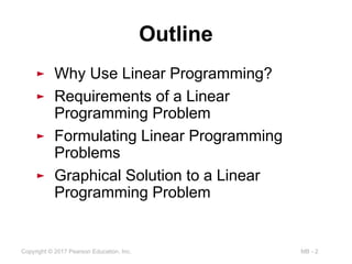
Outline
► Why Use Linear Programming?
► Requirements of a Linear
Programming Problem
► Formulating Linear Programming
Problems
► Graphical Solution to a Linear
Programming Problem
- 3.
MB - 3
Copyright© 2017 Pearson Education, Inc.
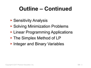
Outline – Continued
▶ Sensitivity Analysis
▶ Solving Minimization Problems
▶ Linear Programming Applications
▶ The Simplex Method of LP
▶ Integer and Binary Variables
- 4.
MB - 4
Copyright© 2017 Pearson Education, Inc.
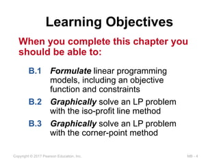
Learning Objectives
When you complete this chapter you
should be able to:
B.1 Formulate linear programming
models, including an objective
function and constraints
B.2 Graphically solve an LP problem
with the iso-profit line method
B.3 Graphically solve an LP problem
with the corner-point method
- 5.
MB - 5
Copyright© 2017 Pearson Education, Inc.
When you complete this chapter you
should be able to:
Learning Objectives
B.4 Interpret sensitivity analysis and
shadow prices
B.5 Construct and solve a minimization
problem
B.6 Formulate production-mix, diet, and
labor scheduling problems
- 6.
MB - 6
Copyright© 2017 Pearson Education, Inc.
Why Use Linear Programming?
▶ A mathematical technique to help plan
and make decisions relative to the
trade-offs necessary to allocate
resources
▶ Will find the minimum or maximum
value of the objective
▶ Guarantees the optimal solution to the
model formulated
- 7.
MB - 7
Copyright© 2017 Pearson Education, Inc.
LP Applications
1. Scheduling school buses to minimize total
distance traveled
2. Allocating police patrol units to high crime
areas in order to minimize response time
to 911 calls
3. Scheduling tellers at banks so that needs
are met during each hour of the day while
minimizing the total cost of labor
- 8.
MB - 8
Copyright© 2017 Pearson Education, Inc.
LP Applications
4. Selecting the product mix in a factory to
make best use of machine- and labor-
hours available while maximizing the
firm’s profit
5. Picking blends of raw materials in feed
mills to produce finished feed
combinations at minimum cost
6. Determining the distribution system that
will minimize total shipping cost
- 9.
MB - 9
Copyright© 2017 Pearson Education, Inc.
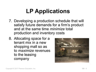
LP Applications
7. Developing a production schedule that will
satisfy future demands for a firm’s product
and at the same time minimize total
production and inventory costs
8. Allocating space for a
tenant mix in a new
shopping mall so as
to maximize revenues
to the leasing
company
- 10.
MB - 10
Copyright© 2017 Pearson Education, Inc.
Requirements of an
LP Problem
1. LP problems seek to maximize or
minimize some quantity (usually
profit or cost) expressed as an
objective function
2. The presence of restrictions, or
constraints, limits the degree to
which we can pursue our objective
- 11.
MB - 11
Copyright© 2017 Pearson Education, Inc.
Requirements of an
LP Problem
3. There must be alternative courses of
action to choose from
4. The objective and constraints in
linear programming problems must
be expressed in terms of linear
equations or inequalities
- 12.
MB - 12
Copyright© 2017 Pearson Education, Inc.
Formulating LP Problems
▶ Glickman Electronics Example
► Two products
1. Glickman x-pod
2. Glickman BlueBerry
► Determine the mix of products that will
produce the maximum profit
- 13.
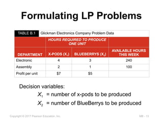
MB - 13
Copyright© 2017 Pearson Education, Inc.
Formulating LP Problems
Decision variables:
X1 = number of x-pods to be produced
X2 = number of BlueBerrys to be produced
TABLE B.1 Glickman Electronics Company Problem Data
HOURS REQUIRED TO PRODUCE
ONE UNIT
DEPARTMENT X-PODS (X1) BLUEBERRYS (X2)
AVAILABLE HOURS
THIS WEEK
Electronic 4 3 240
Assembly 2 1 100
Profit per unit $7 $5
- 14.
MB - 14
Copyright© 2017 Pearson Education, Inc.
Formulating LP Problems
Objective function:
Maximize profit = $7X1 + $5X2
There are three types of constraints
► Upper limits (LHS ≤ RHS) where the total amount
used cannot exceed the availability of that resource
► Lower limits (LHS ≥ RHS) where the amount of the
resource used cannot be less than a specified
amount
► Equalities (LHS = RHS) where all of a resource
must be used
- 15.
MB - 15
Copyright© 2017 Pearson Education, Inc.
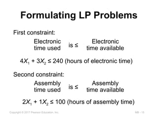
Formulating LP Problems
Second constraint:
2X1 + 1X2 ≤ 100 (hours of assembly time)
Assembly
time available
Assembly
time used is ≤
First constraint:
4X1 + 3X2 ≤ 240 (hours of electronic time)
Electronic
time available
Electronic
time used is ≤
- 16.
MB - 16
Copyright© 2017 Pearson Education, Inc.
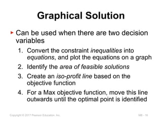
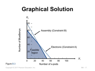
Graphical Solution
▶ Can be used when there are two decision
variables
1. Convert the constraint inequalities into
equations, and plot the equations on a graph
2. Identify the area of feasible solutions
3. Create an iso-profit line based on the
objective function
4. For a Max objective function, move this line
outwards until the optimal point is identified
- 17.
MB - 17
Copyright© 2017 Pearson Education, Inc.
Graphical Solution
100 –
–
80 –
–
60 –
–
40 –
–
20 –
–
–
| | | | | | | | | | |
0 20 40 60 80 100
Number
of
BlueBerrys
Number of x-pods
X1
X2
Assembly (Constraint B)
Electronic (Constraint A)
Feasible
region
Figure B.3
- 18.
MB - 18
Copyright© 2017 Pearson Education, Inc.
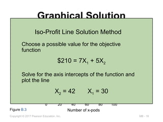
Graphical Solution
100 –
–
80 –
–
60 –
–
40 –
–
20 –
–
–
| | | | | | | | | | |
0 20 40 60 80 100
Number
of
BlueBerrys
Number of x-pods
X1
X2
Assembly (Constraint B)
Electronic (Constraint A)
Feasible
region
Figure B.3
Iso-Profit Line Solution Method
Choose a possible value for the objective
function
$210 = 7X1 + 5X2
Solve for the axis intercepts of the function and
plot the line
X2 = 42 X1 = 30
- 19.
MB - 19
Copyright© 2017 Pearson Education, Inc.
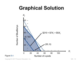
Graphical Solution
100 –
–
80 –
–
60 –
–
40 –
–
20 –
–
–
| | | | | | | | | | |
0 20 40 60 80 100
Number
of
BlueBerrys
Number of x-pods
X1
X2
Figure B.4
(0, 42)
(30, 0)
$210 = $7X1 + $5X2
- 20.
MB - 20
Copyright© 2017 Pearson Education, Inc.
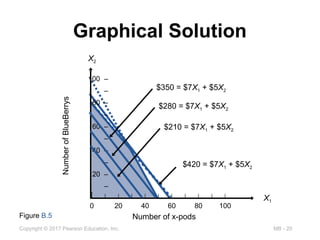
Graphical Solution
100 –
–
80 –
–
60 –
–
40 –
–
20 –
–
–
| | | | | | | | | | |
0 20 40 60 80 100
Number
of
BlueBerrys
Number of x-pods
X1
X2
Figure B.5
$210 = $7X1 + $5X2
$420 = $7X1 + $5X2
$350 = $7X1 + $5X2
$280 = $7X1 + $5X2
- 21.
MB - 21
Copyright© 2017 Pearson Education, Inc.
Graphical Solution
100 –
–
80 –
–
60 –
–
40 –
–
20 –
–
–
| | | | | | | | | | |
0 20 40 60 80 100
Number
of
BlueBerrys
Number of x-pods
X1
X2
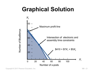
$410 = $7X1 + $5X2
Maximum profit line
Intersection of electronic and
assembly time constraints
- 22.
MB - 22
Copyright© 2017 Pearson Education, Inc.
Graphical Solution
100 –
–
80 –
–
60 –
–
40 –
–
20 –
–
–
| | | | | | | | | | |
0 20 40 60 80 100
Number
of
BlueBerrys
Number of x-pods
X1
X2
$410 = $7X1 + $5X2
Maximum profit line
Intersection of electronic and
assembly time constraints
2
3
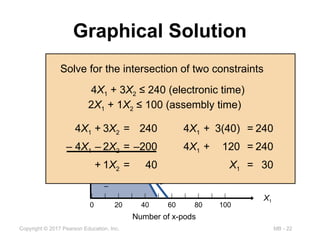
Solve for the intersection of two constraints
2X1 + 1X2 ≤ 100 (assembly time)
4X1 + 3X2 ≤ 240 (electronic time)
4X1 + 3X2 = 240
– 4X1 – 2X2 = –200
+ 1X2 = 40
4X1 + 3(40) = 240
4X1 + 120 = 240
X1 = 30
- 23.
MB - 23
Copyright© 2017 Pearson Education, Inc.
Graphical Solution
100 –
–
80 –
–
60 –
–
40 –
–
20 –
–
–
| | | | | | | | | | |
0 20 40 60 80 100
Number
of
BlueBerrys
Number of x-pods
X1
X2
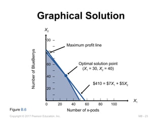
Figure B.6
$410 = $7X1 + $5X2
Maximum profit line
Optimal solution point
(X1 = 30, X2 = 40)
- 24.
MB - 24
Copyright© 2017 Pearson Education, Inc.
100 –
–
80 –
–
60 –
–
40 –
–
20 –
–
–
| | | | | | | | | | |
0 20 40 60 80 100
Number
of
BlueBerrys
Number of x-pods
X1
X2
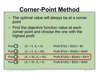
Corner-Point Method
Figure B.7
1
2
3
4
- 25.
MB - 25
Copyright© 2017 Pearson Education, Inc.
100 –
–
80 –
–
60 –
–
40 –
–
20 –
–
–
| | | | | | | | | | |
0 20 40 60 80 100
Number
of
BlueBerrys
Number of x-pods
X1
X2
Corner-Point Method
Figure B.7
1
2
3
4
► The optimal value will always be at a corner
point
► Find the objective function value at each
corner point and choose the one with the
highest profit
Point 1 : (X1 = 0, X2 = 0) Profit $7(0) + $5(0) = $0
Point 2 : (X1 = 0, X2 = 80) Profit $7(0) + $5(80) = $400
Point 3 : (X1 = 30, X2 = 40) Profit $7(30) + $5(40) = $410
Point 4 : (X1 = 50, X2 = 0) Profit $7(50) + $5(0) = $350
- 26.
MB - 26
Copyright© 2017 Pearson Education, Inc.
Sensitivity Analysis
▶ How sensitive the results are to
parameter changes
▶ Change in the value of coefficients
▶ Change in a right-hand-side value of a
constraint
▶ Trial-and-error approach
▶ Analytic postoptimality method
- 27.
- 28.
MB - 28
Copyright© 2017 Pearson Education, Inc.
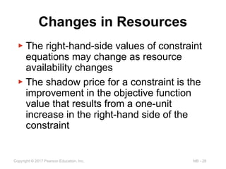
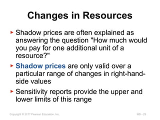
Changes in Resources
▶ The right-hand-side values of constraint
equations may change as resource
availability changes
▶ The shadow price for a constraint is the
improvement in the objective function
value that results from a one-unit
increase in the right-hand side of the
constraint
- 29.
MB - 29
Copyright© 2017 Pearson Education, Inc.
Changes in Resources
▶ Shadow prices are often explained as
answering the question "How much would
you pay for one additional unit of a
resource?"
▶ Shadow prices are only valid over a
particular range of changes in right-hand-
side values
▶ Sensitivity reports provide the upper and
lower limits of this range
- 30.
MB - 30
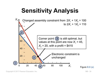
Copyright© 2017 Pearson Education, Inc.
Sensitivity Analysis
–
100 –
–
80 –
–
60 –
–
40 –
–
20 –
–
–
| | | | | | | | | | |
0 20 40 60 80 100 X1
X2
Figure B.8 (a)
Changed assembly constraint from 2X1 + 1X2 = 100
to 2X1 + 1X2 = 110
Electronic constraint is
unchanged
Corner point 3 is still optimal, but
values at this point are now X1 = 45,
X2 = 20, with a profit = $415
1
2
3
4
- 31.
MB - 31
Copyright© 2017 Pearson Education, Inc.
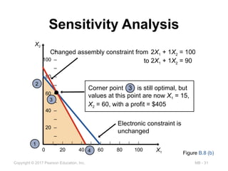
Sensitivity Analysis
–
100 –
–
80 –
–
60 –
–
40 –
–
20 –
–
–
| | | | | | | | | | |
0 20 40 60 80 100 X1
X2
Figure B.8 (b)
Electronic constraint is
unchanged
Corner point 3 is still optimal, but
values at this point are now X1 = 15,
X2 = 60, with a profit = $405
1
2
3
4
Changed assembly constraint from 2X1 + 1X2 = 100
to 2X1 + 1X2 = 90
- 32.
MB - 32
Copyright© 2017 Pearson Education, Inc.
Changes in the
Objective Function
▶ A change in the coefficients in the
objective function may cause a different
corner point to become the optimal
solution
▶ The sensitivity report shows how much
objective function coefficients may
change without changing the optimal
solution point
- 33.
MB - 33
Copyright© 2017 Pearson Education, Inc.
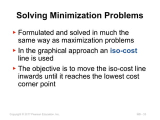
Solving Minimization Problems
▶ Formulated and solved in much the
same way as maximization problems
▶ In the graphical approach an iso-cost
line is used
▶ The objective is to move the iso-cost line
inwards until it reaches the lowest cost
corner point
- 34.
MB - 34
Copyright© 2017 Pearson Education, Inc.
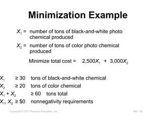
Minimization Example
X1 = number of tons of black-and-white photo
chemical produced
X2 = number of tons of color photo chemical
produced
Minimize total cost = 2,500X1 + 3,000X2
X1 ≥ 30 tons of black-and-white chemical
X2 ≥ 20 tons of color chemical
X1 + X2 ≥ 60 tons total
X1, X2 ≥ $0 nonnegativity requirements
- 35.
MB - 35
Copyright© 2017 Pearson Education, Inc.
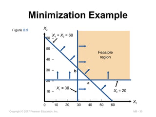
Minimization Example
Figure B.9
60 –
50 –
40 –
30 –
20 –
10 –
–
| | | | | | |
0 10 20 30 40 50 60
X1
X2
Feasible
region
X1 = 30
X2 = 20
X1 + X2 = 60
b
a
- 36.
MB - 36
Copyright© 2017 Pearson Education, Inc.
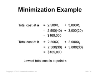
Minimization Example
Total cost at a = 2,500X1 + 3,000X2
= 2,500(40) + 3,000(20)
= $160,000
Total cost at b = 2,500X1 + 3,000X2
= 2,500(30) + 3,000(30)
= $165,000
Lowest total cost is at point a
- 37.
MB - 37
Copyright© 2017 Pearson Education, Inc.
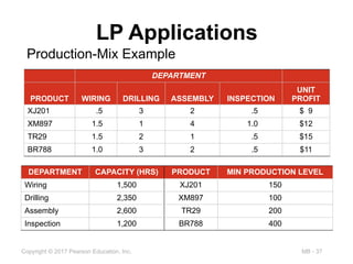
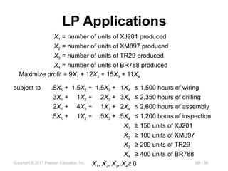
LP Applications
Production-Mix Example
DEPARTMENT
PRODUCT WIRING DRILLING ASSEMBLY INSPECTION
UNIT
PROFIT
XJ201 .5 3 2 .5 $ 9
XM897 1.5 1 4 1.0 $12
TR29 1.5 2 1 .5 $15
BR788 1.0 3 2 .5 $11
DEPARTMENT CAPACITY (HRS) PRODUCT MIN PRODUCTION LEVEL
Wiring 1,500 XJ201 150
Drilling 2,350 XM897 100
Assembly 2,600 TR29 200
Inspection 1,200 BR788 400
- 38.
MB - 38
Copyright© 2017 Pearson Education, Inc.
LP Applications
X1 = number of units of XJ201 produced
X2 = number of units of XM897 produced
X3 = number of units of TR29 produced
X4 = number of units of BR788 produced
Maximize profit = 9X1 + 12X2 + 15X3 + 11X4
subject to .5X1 + 1.5X2 + 1.5X3 + 1X4 ≤ 1,500 hours of wiring
3X1 + 1X2 + 2X3 + 3X4 ≤ 2,350 hours of drilling
2X1 + 4X2 + 1X3 + 2X4 ≤ 2,600 hours of assembly
.5X1 + 1X2 + .5X3 + .5X4 ≤ 1,200 hours of inspection
X1 ≥ 150 units of XJ201
X2 ≥ 100 units of XM897
X3 ≥ 200 units of TR29
X4 ≥ 400 units of BR788
X1, X2, X3, X4≥ 0
- 39.
MB - 39
Copyright© 2017 Pearson Education, Inc.
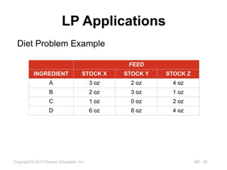
LP Applications
Diet Problem Example
FEED
INGREDIENT STOCK X STOCK Y STOCK Z
A 3 oz 2 oz 4 oz
B 2 oz 3 oz 1 oz
C 1 oz 0 oz 2 oz
D 6 oz 8 oz 4 oz
- 40.
MB - 40
Copyright© 2017 Pearson Education, Inc.
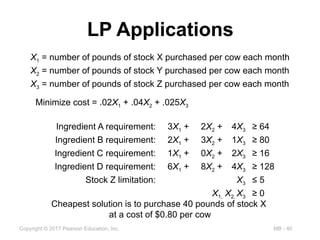
LP Applications
X1 = number of pounds of stock X purchased per cow each month
X2 = number of pounds of stock Y purchased per cow each month
X3 = number of pounds of stock Z purchased per cow each month
Minimize cost = .02X1 + .04X2 + .025X3
Ingredient A requirement: 3X1 + 2X2 + 4X3 ≥ 64
Ingredient B requirement: 2X1 + 3X2 + 1X3 ≥ 80
Ingredient C requirement: 1X1 + 0X2 + 2X3 ≥ 16
Ingredient D requirement: 6X1 + 8X2 + 4X3 ≥ 128
Stock Z limitation: X3 ≤ 5
X1, X2, X3 ≥ 0
Cheapest solution is to purchase 40 pounds of stock X
at a cost of $0.80 per cow
- 41.
MB - 41
Copyright© 2017 Pearson Education, Inc.
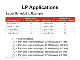
LP Applications
Labor Scheduling Example
F = Full-time tellers
P1 = Part-time tellers starting at 9 AM (leaving at 1 PM)
P2 = Part-time tellers starting at 10 AM (leaving at 2 PM)
P3 = Part-time tellers starting at 11 AM (leaving at 3 PM)
P4 = Part-time tellers starting at noon (leaving at 4 PM)
P5 = Part-time tellers starting at 1 PM (leaving at 5 PM)
TIME PERIOD
NUMBER OF
TELLERS REQUIRED TIME PERIOD
NUMBER OF
TELLERS REQUIRED
9 a.m.–10 a.m. 10 1 p.m.–2 p.m. 18
10 a.m.–11 a.m. 12 2 p.m.–3 p.m. 17
11 a.m.–Noon 14 3 p.m.–4 p.m. 15
Noon–1 p.m. 16 4 p.m.–5 p.m. 10
- 42.
MB - 42
Copyright© 2017 Pearson Education, Inc.
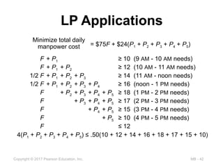
LP Applications
= $75F + $24(P1 + P2 + P3 + P4 + P5)
Minimize total daily
manpower cost
F + P1 ≥ 10 (9 AM - 10 AM needs)
F + P1 + P2 ≥ 12 (10 AM - 11 AM needs)
1/2 F + P1 + P2 + P3 ≥ 14 (11 AM - noon needs)
1/2 F + P1 + P2 + P3 + P4 ≥ 16 (noon - 1 PM needs)
F + P2 + P3 + P4 + P5 ≥ 18 (1 PM - 2 PM needs)
F + P3 + P4 + P5 ≥ 17 (2 PM - 3 PM needs)
F + P4 + P5 ≥ 15 (3 PM - 4 PM needs)
F + P5 ≥ 10 (4 PM - 5 PM needs)
F ≤ 12
4(P1 + P2 + P3 + P4 + P5) ≤ .50(10 + 12 + 14 + 16 + 18 + 17 + 15 + 10)
- 43.
MB - 43
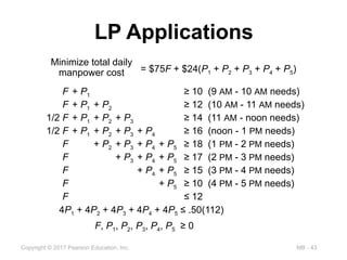
Copyright© 2017 Pearson Education, Inc.
LP Applications
= $75F + $24(P1 + P2 + P3 + P4 + P5)
Minimize total daily
manpower cost
F + P1 ≥ 10 (9 AM - 10 AM needs)
F + P1 + P2 ≥ 12 (10 AM - 11 AM needs)
1/2 F + P1 + P2 + P3 ≥ 14 (11 AM - noon needs)
1/2 F + P1 + P2 + P3 + P4 ≥ 16 (noon - 1 PM needs)
F + P2 + P3 + P4 + P5 ≥ 18 (1 PM - 2 PM needs)
F + P3 + P4 + P5 ≥ 17 (2 PM - 3 PM needs)
F + P4 + P5 ≥ 15 (3 PM - 4 PM needs)
F + P5 ≥ 10 (4 PM - 5 PM needs)
F ≤ 12
4P1 + 4P2 + 4P3 + 4P4 + 4P5 ≤ .50(112)
F, P1, P2, P3, P4, P5 ≥ 0
- 44.
MB - 44
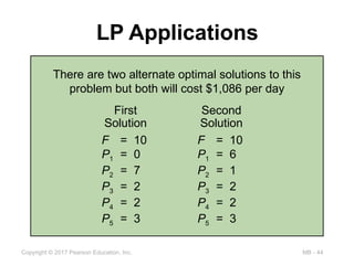
Copyright© 2017 Pearson Education, Inc.
LP Applications
There are two alternate optimal solutions to this
problem but both will cost $1,086 per day
F = 10 F = 10
P1 = 0 P1 = 6
P2 = 7 P2 = 1
P3 = 2 P3 = 2
P4 = 2 P4 = 2
P5 = 3 P5 = 3
First Second
Solution Solution
- 45.
MB - 45
Copyright© 2017 Pearson Education, Inc.
The Simplex Method
▶ Real world problems are too complex to
be solved using the graphical method
▶ The simplex method is an algorithm for
solving more complex problems
▶ Developed by George Dantzig in the late
1940s
▶ Most computer-based LP packages use
the simplex method
- 46.
MB - 46
Copyright© 2017 Pearson Education, Inc.
Integer and Binary Variables
▶ In some cases solutions must be integers
▶ Binary variables allow for “yes-or-no”
decisions
▶ Not good practice to round variables to
integers
▶ Constraints can be added to force integer
or binary values
▶ Larger programs may take longer to solve
- 47.
MB - 47
Copyright© 2017 Pearson Education, Inc.
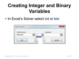
Creating Integer and Binary
Variables
▶ In Excel’s Solver select int or bin
- 48.
MB - 48
Copyright© 2017 Pearson Education, Inc.
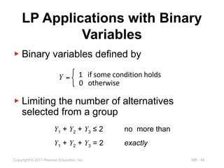
LP Applications with Binary
Variables
▶ Binary variables defined by
▶ Limiting the number of alternatives
selected from a group
Y1 + Y2 + Y3 ≤ 2 no more than
Y1 + Y2 + Y3 = 2 exactly
- 49.
MB - 49
Copyright© 2017 Pearson Education, Inc.
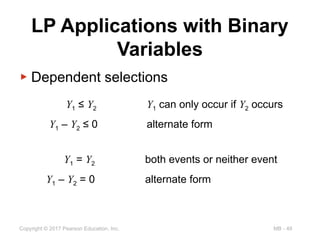
LP Applications with Binary
Variables
▶ Dependent selections
Y1 ≤ Y2 Y1 can only occur if Y2 occurs
Y1 – Y2 ≤ 0 alternate form
Y1 = Y2 both events or neither event
Y1 – Y2 = 0 alternate form
- 50.
MB - 50
Copyright© 2017 Pearson Education, Inc.
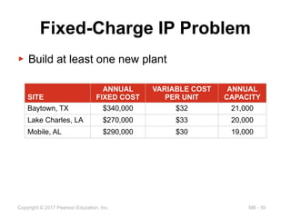
Fixed-Charge IP Problem
▶ Build at least one new plant
SITE
ANNUAL
FIXED COST
VARIABLE COST
PER UNIT
ANNUAL
CAPACITY
Baytown, TX $340,000 $32 21,000
Lake Charles, LA $270,000 $33 20,000
Mobile, AL $290,000 $30 19,000
- 51.
MB - 51
Copyright© 2017 Pearson Education, Inc.
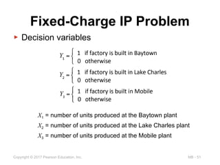
Fixed-Charge IP Problem
▶ Decision variables
X1 = number of units produced at the Baytown plant
X2 = number of units produced at the Lake Charles plant
X3 = number of units produced at the Mobile plant
- 52.
MB - 52
Copyright© 2017 Pearson Education, Inc.
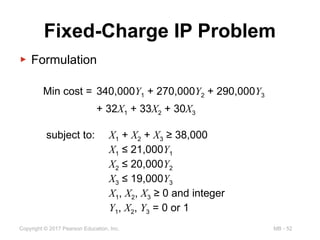
Fixed-Charge IP Problem
▶ Formulation
Min cost = 340,000Y1 + 270,000Y2 + 290,000Y3
+ 32X1 + 33X2 + 30X3
subject to: X1 + X2 + X3 ≥ 38,000
X1 ≤ 21,000Y1
X2 ≤ 20,000Y2
X3 ≤ 19,000Y3
X1, X2, X3 ≥ 0 and integer
Y1, X2, Y3 = 0 or 1
- 53.
MB - 53
Copyright© 2017 Pearson Education, Inc.
All rights reserved. No part of this publication may be reproduced, stored in a
retrieval system, or transmitted, in any form or by any means, electronic,
mechanical, photocopying, recording, or otherwise, without the prior written
permission of the publisher.
Printed in the United States of America.
Editor's Notes
- #33 It might be useful at this point to discuss typical equipment utilization rates for different process strategies if you have not done so before.
- #34 It might be useful at this point to discuss typical equipment utilization rates for different process strategies if you have not done so before.
- #35 It might be useful at this point to discuss typical equipment utilization rates for different process strategies if you have not done so before.
- #36 It might be useful at this point to discuss typical equipment utilization rates for different process strategies if you have not done so before.