chapter 2: LINEAR PROGRAMMING FORMULATION AND SOLUTION

CHAPTER TWO
LINEAR PROGRAMMING
MODEL

Definitions of Linear
Programming(LP)
 Linear programming uses a mathematical model to find the
best allocation of scarce resources to various activities so as
to maximize profit or minimize cost.
 Linear programming is used to find the best (Optimal
solution) to a problem that requires a decision about how
best to use a set of limited resources to achieve objectives.
 Linear Programming is applied for determining the
optimal allocation of re
sources like raw materials,
machines, manpower, etc. by a firm

Meaning of linear programming
 The term “Linear Programming” consists of two words as linear and
programming. The word “linear” defines the relationship between
multiple variables with degree one. The word “programming” defines
the process of selecting the best solution from various alternatives.
 Thus, Linear programming is a mathematical model used to solve
problems that can be represented by a system of linear equations and
inequalities.
 Both the objective function and the constraints must be formulated in
terms of a linear equality or inequality.
1–3

Applications of linear programming problem
 Product mix: is used when a company produce several different products,
each of which requires the use of limited production resources such as raw
material, labour, and equipment
 Linear programming is to determine the quantity of each product to be
produced to maximize the company’s profit or minimize its cost.
 Blending problems: Blending problems refer to situations in which a number
of components (or commodities) are mixed together to yield one or more
products.
 The objective here is to determine how much of each commodity should be
purchased and blended

Applications of linear programming problem
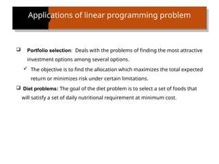
 Portfolio selection: Deals with the problems of finding the most attractive
investment options among several options.
 The objective is to find the allocation which maximizes the total expected
return or minimizes risk under certain limitations.
 Diet problems: The goal of the diet problem is to select a set of foods that
will satisfy a set of daily nutritional requirement at minimum cost.

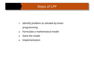
1) Identify problem as solvable by linear
programming
2) Formulate a mathematical model
3) Solve the model
4) Implementation
Steps of LPP

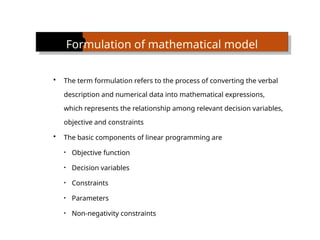
Formulation of mathematical model
 The term formulation refers to the process of converting the verbal
description and numerical data into mathematical expressions,
which represents the relationship among relevant decision variables,
objective and constraints
 The basic components of linear programming are
• Objective function
• Decision variables
• Constraints
• Parameters
• Non-negativity constraints

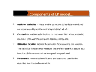
Components of LP model…
 Decision Variables – These are the quantities to be determined and
are represented by mathematical symbols (x1,x2,x3…)
 Constraints – refers to limitations on resources like Labour, material,
machine, time, warehouse space, capital, energy, etc.
 Objective function defines the criterion for evaluating the solution.
The objective function may measure the profit or cost that occurs as a
function of the amounts of various products produced.
 Parameters - numerical coefficients and constants used in the
objective function and constraints.

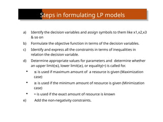
Steps in formulating LP models
a) Identify the decision variables and assign symbols to them like x1,x2,x3
& so on
b) Formulate the objective function in terms of the decision variables.
c) Identify and express all the constraints in terms of inequalities in
relation the decision variable.
d) Determine appropriate values for parameters and determine whether
an upper limit( ), lower limit( ), or equality(=) is called for.
≤ ≥
 ≤ is used if maximum amount of a resource is given (Maximization
case)
 ≥ is used if the minimum amount of resource is given (Minimization
case)
 = is used if the exact amount of resource is known
e) Add the non-negativity constraints.

Linear programming model format

formulation…
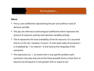
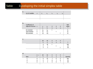
Where,
 The cj s are coefficients representing the per unit profit (or cost) of
decision variable
 The aij’s are referred as technological coefficients which represent the
amount of resource used by each decision variable( activity)
 The bi represents the total availability of the ith resource. It is assumed
that bi 0 for all i. However, if any bi < 0, then both sides of constraint i
≥
is multiplied by –1 to make bi > 0 and reverse the inequality of the
constraint.
 The expression ( , =, ) means that in any specific problem each
≤ ≥
constraint may take only one of the three possible forms: (i) less than or
equal to ( ) (ii) equal to (=) (iii) greater than or equal to ( )
≤ ≥

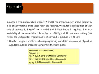
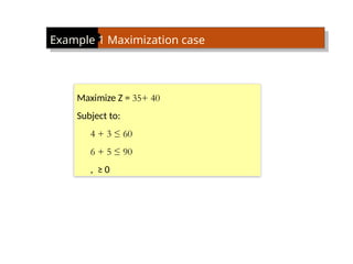
Example 1
Suppose a firm produces two products A and B. For producing each unit of product A,
4 Kg of Raw material and 6 labor hours are required. While, for the production of each
unit of product B, 3 kg of raw material and 5 labor hours is required. The total
availability of raw material and labor hours is 60 Kg and 90 Hours respectively (per
week). The unit profit of Product A LP is 35 Birr and of product, B is 40 Birr.
 Develop the given problem as linear programing and determine amount of product
A and B should be produced to maximize the firm’s profit.
Maximize Z = 35x1+ 40x2
Subject to:
4x1 + 3,x2 ≤ 60 (Raw Material Constraint)
6x1, + 5x2 ≤ 90 (Labor Hours Constraint)
x1, x2 ≥ 0 (Non-negativity Constraint)

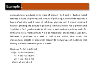
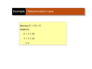
A manufacturer produces three types of product A, B and c. Each A model
requires 4 hours of grinding and 2 hours of polishing; each B model requires 2
hours of grinding and 5 hours of polishing. whereas each C model requires 3
hours of grinding and 3 hours of polishing The manufacturer has 2 grinders and
3 polishers. Each grinder works for 40 hours a week and each polisher works for
60 hours a week. Profit on model A is 3, on model B is 4 and on model C is 5 birr. .
Whatever is produced in a week is sold in the market. How should the
manufacturer allocate his production capacity to the two types of models so that
he may make the maximum profit in a week?
Maximize Z = 3x1 + 4x2+ 5x3
subject to the constraints:
4x1 + 2x2 + 3x3 80
≤
2x1 + 5x2 +3x3 180
≤
Where, x1 and x2 0
≥
Example 2

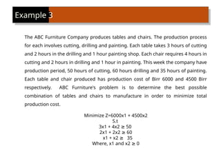
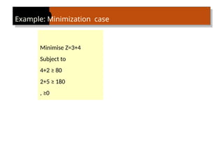
The ABC Furniture Company produces tables and chairs. The production process
for each involves cutting, drilling and painting. Each table takes 3 hours of cutting
and 2 hours in the drilling and 1 hour painting shop. Each chair requires 4 hours in
cutting and 2 hours in drilling and 1 hour in painting. This week the company have
production period, 50 hours of cutting, 60 hours drilling and 35 hours of painting.
Each table and chair produced has production cost of Birr 6000 and 4500 Birr
respectively. ABC Furniture's problem is to determine the best possible
combination of tables and chairs to manufacture in order to minimize total
production cost.
Minimize Z=6000x1 + 4500x2
S.t
3x1 + 4x2 50
≥
2x1 + 2x2 60
≥
x1 + x2 35
≥
Where, x1 and x2 0
≥
Example 3

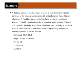
• A dietician wishes to mix two types of foods in such a way that vitamin
contents of the mixture contain at least 8 units of vitamin A and 10 units
of vitamin C. Food I contains 2 units/kg of vitamin A and 1 unit/kg of
vitamin C. Food II contains 1 unit/kg of vitamin A and 2 units/kg of vitamin
C. It costs birr 50 per kg to purchase Food I and birr .70 per kg to purchase
Food II. Formulate this problem as a linear programming problem to
minimise the cost of such a mixture.
Minimise Z=50x1+70x2
subject to the constraints
2x1+x2 8
≥
x1+2x2 10
≥
x1,x2 0
≥
Example 4

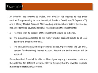
An investor has 100,000 to invest. The investor has decided to use three
vehicles for generating income: Municipal Bonds, a Certificate Of Deposit (CD),
and a Money Market Account. After reading a financial newsletter, the investor
has also identified several additional restrictions on the investments:
a) No more than 40 percent of the investment should be in bonds.
b) The proportion allocated to the money market account should be at least
double the amount in the CD.
c) The annual return will be 8 percent for bonds, 9 percent for the CD, and 7
percent for the money market account. Assume the entire amount will be
invested.
Formulate the LP model for this problem, ignoring any transaction costs and
the potential for different investment lives. Assume that the investor wants to
maximize the total annual return.
Example 5

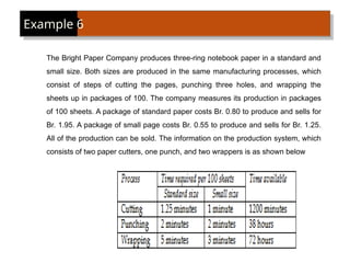
The Bright Paper Company produces three-ring notebook paper in a standard and
small size. Both sizes are produced in the same manufacturing processes, which
consist of steps of cutting the pages, punching three holes, and wrapping the
sheets up in packages of 100. The company measures its production in packages
of 100 sheets. A package of standard paper costs Br. 0.80 to produce and sells for
Br. 1.95. A package of small page costs Br. 0.55 to produce and sells for Br. 1.25.
All of the production can be sold. The information on the production system, which
consists of two paper cutters, one punch, and two wrappers is as shown below
Example 6

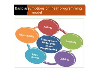
Basic assumptions of linear programming
model

Assumptions of linear programming…
1. Proportionality/ Linearity: any change in the constraint inequalities will
have the proportional change in the objective function. Thus, if the output is
doubled, the profit would also be doubled.
2. Additivity: the total profit of the objective function is determined by the sum
of profit contributed by each product separately. Similarly, the total amount
of resources used is determined by the sum of resources used by each
product separately.
3. Divisibility /continuity: the values of decision variables can be fractions
although fraction values have no sense sometimes
4. Certainty: the parameters of objective function coefficients and the
coefficients of constraint inequalities is known with certainty. Such as profit
per unit of product, availability of material and labor per unit, requirement of
material and labor per unit are known and is given in the linear programming
problem.
5. Finite Choices: the decision variables assume non-negative values b/c the
output in the production problem can not be negative.

Solving Linear Programming Problems
There are generally two methods of solving LPP
• Graphic method
• Simplex method

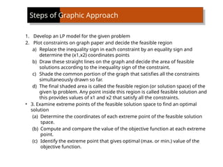
Steps of Graphic Approach
1. Develop an LP model for the given problem
2. Plot constraints on graph paper and decide the feasible region
a) Replace the inequality sign in each constraint by an equality sign and
determine the (x1,x2) coordinates points
b) Draw these straight lines on the graph and decide the area of feasible
solutions according to the inequality sign of the constraint.
c) Shade the common portion of the graph that satisfies all the constraints
simultaneously drawn so far.
d) The final shaded area is called the feasible region (or solution space) of the
given lp problem. Any point inside this region is called feasible solution and
this provides values of x1 and x2 that satisfy all the constraints.
• 3. Examine extreme points of the feasible solution space to find an optimal
solution
(a) Determine the coordinates of each extreme point of the feasible solution
space.
(b) Compute and compare the value of the objective function at each extreme
point.
(c) Identify the extreme point that gives optimal (max. or min.) value of the
objective function.

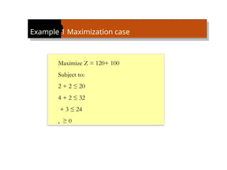
Example 1 Maximization case
Maximize Z = 35+ 40
Subject to:
4 + 3 ≤ 60
6 + 5 ≤ 90
, ≥ 0

Maximize Z = 10+ 15
Subject to:
6 + 3 ≤ 48
3 + 5 ≤ 60
, ≥ 0

Example: Minimization case
Minimise Z=3+4
Subject to
4+2 ≥ 80
2+5 ≥ 180
, ≥0

Maximize Z = 120+ 100
Subject to:
2 + 2 ≤ 20
4 + 2 ≤ 32
+ 3 ≤ 24
, ≥ 0

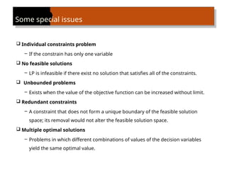
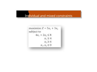
Some special issues
 Individual constraints problem
– If the constrain has only one variable
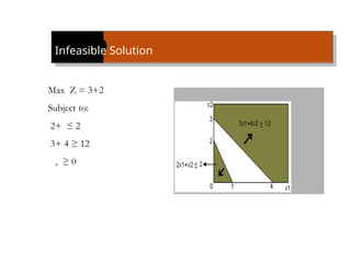
 No feasible solutions
– LP is infeasible if there exist no solution that satisfies all of the constraints.
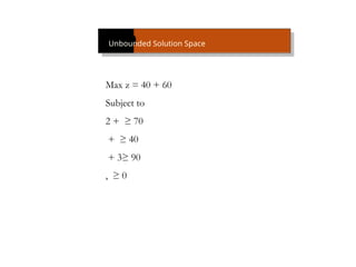
 Unbounded problems
– Exists when the value of the objective function can be increased without limit.
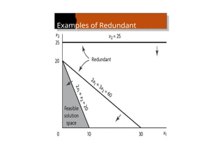
 Redundant constraints
– A constraint that does not form a unique boundary of the feasible solution
space; its removal would not alter the feasible solution space.
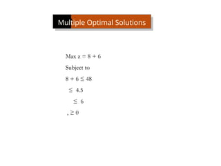
 Multiple optimal solutions
– Problems in which different combinations of values of the decision variables
yield the same optimal value.

Infeasible Solution
Max Z = 3+2
Subject to:
2+ ≤ 2
3+ 4 ≥ 12
, ≥ 0

An Unbounded Solution Space
Max z = 40 + 60
Subject to
2 + ≥ 70
+ ≥ 40
+ 3≥ 90
, ≥ 0

Examples of Redundant
Constraints

Multiple Optimal Solutions
Max z = 8 + 6
Subject to
8 + 6 ≤ 48
≤ 4.5
≤ 6
, ≥ 0

Individual and mixed constraints

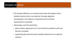
– The Simplex Method is an iterative technique that begins with a
feasible solution that is not optimal, through algebraic
manipulation, the solution is improved until no further
improvement is possible.
– Advantages and Characteristics
• More realistic approach as it is not limited to problems with two
decision variables
• Systematically examines basic feasible solutions for an optimal
solution.
Simplex Method

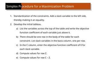
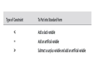
Simplex Procedure for a Maximization Problem
1. Standardization of the constraints. Add a slack variable to the left side,
thereby making it an equality.
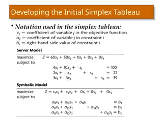
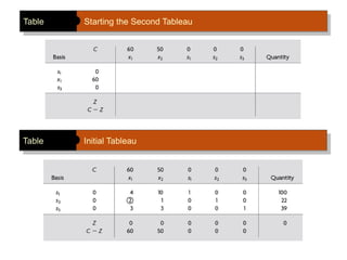
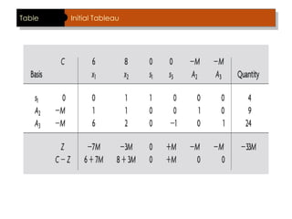
2. Develop the initial tableau.
a) List the variables across the top of the table and write the objective
function coefficient of each variable just above it.
b) There should be one row in the body of the table for each
constraint. List slack variables in the basis column, one per row.
c) In the C column, enter the objective function coefficient of 0 for
each slack variable.
d) Compute values for row Z.
e) Compute values for row C – Z.

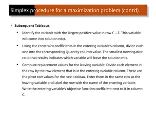
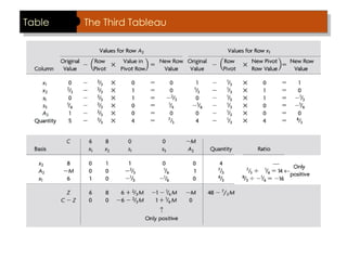
Simplex procedure for a maximization problem (cont’d)
• Subsequent Tableaus
 Identify the variable with the largest positive value in row C – Z. This variable
will come into solution next.
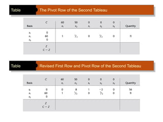
 Using the constraint coefficients in the entering variable’s column, divide each
one into the corresponding Quantity column value. The smallest nonnegative
ratio that results indicates which variable will leave the solution mix.
 Compute replacement values for the leaving variable: Divide each element in
the row by the row element that is in the entering variable column. These are
the pivot row values for the next tableau. Enter them in the same row as the
leaving variable and label the row with the name of the entering variable.
Write the entering variable’s objective function coefficient next to it in column
C.

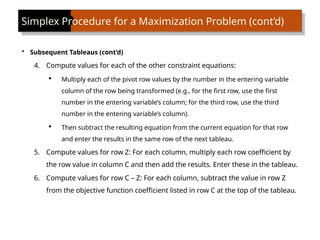
Simplex Procedure for a Maximization Problem (cont’d)
• Subsequent Tableaus (cont’d)
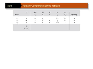
4. Compute values for each of the other constraint equations:
 Multiply each of the pivot row values by the number in the entering variable
column of the row being transformed (e.g., for the first row, use the first
number in the entering variable’s column; for the third row, use the third
number in the entering variable’s column).
 Then subtract the resulting equation from the current equation for that row
and enter the results in the same row of the next tableau.
5. Compute values for row Z: For each column, multiply each row coefficient by
the row value in column C and then add the results. Enter these in the tableau.
6. Compute values for row C – Z: For each column, subtract the value in row Z
from the objective function coefficient listed in row C at the top of the tableau.

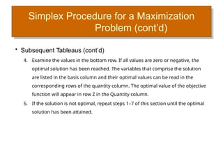
Simplex Procedure for a Maximization
Problem (cont’d)
• Subsequent Tableaus (cont’d)
4. Examine the values in the bottom row. If all values are zero or negative, the
optimal solution has been reached. The variables that comprise the solution
are listed in the basis column and their optimal values can be read in the
corresponding rows of the quantity column. The optimal value of the objective
function will appear in row Z in the Quantity column.
5. If the solution is not optimal, repeat steps 1–7 of this section until the optimal
solution has been attained.

Developing the Initial Simplex Tableau
• Notation used in the simplex tableau:

Table Developing the initial simplex table

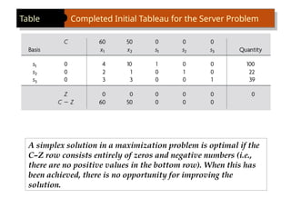
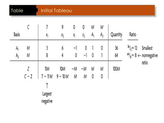
Table Completed Initial Tableau for the Server Problem
A simplex solution in a maximization problem is optimal if the
C–Z row consists entirely of zeros and negative numbers (i.e.,
there are no positive values in the bottom row). When this has
been achieved, there is no opportunity for improving the
solution.

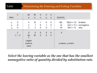
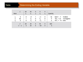
Table Determining the Entering and Exiting Variables
Select the leaving variable as the one that has the smallest
nonnegative ratio of quantity divided by substitution rate.

Table Starting the Second Tableau
Table Initial Tableau

Table The Pivot Row of the Second Tableau
Table Revised First Row and Pivot Row of the Second Tableau

Table Partially Completed Second Tableau

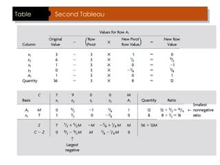
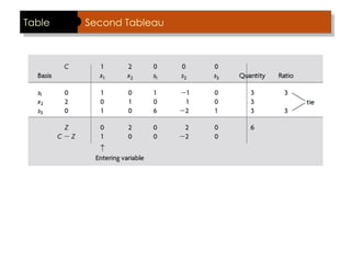
Table Completed Second Tableau
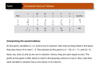
Interpreting the second tableau
At this point, variables s1, x1, and s3 are in solution. Not only are they listed in the basis,
they also have a 0 in row C – Z. The solution at this point is s1 = 56, x1 = 11, and s3 = 6.
Note, too, that x2 and s2 are not in solution. Hence, they are each equal to zero. The
profit at this point is 660, which is read in the Quantity column in row Z. Also, note that
each variable in solution has a unit vector in its column.

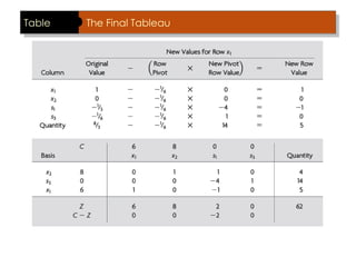
Table Determining the Exiting Variable

Table Pivot Row Values for the Third Tableau
Table Partially Completed Third Tableau

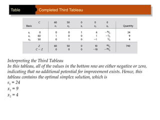
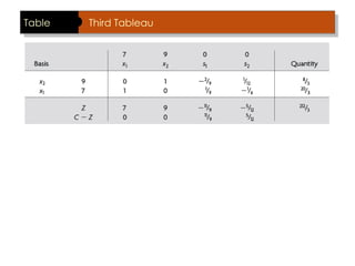
Table Completed Third Tableau
Interpreting the Third Tableau
In this tableau, all of the values in the bottom row are either negative or zero,
indicating that no additional potential for improvement exists. Hence, this
tableau contains the optimal simplex solution, which is
s1 = 24
x1 = 9
x2 = 4

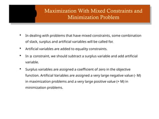
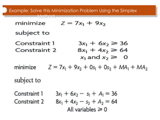
Maximization With Mixed Constraints and
Minimization Problem
 In dealing with problems that have mixed constraints, some combination
of slack, surplus and artificial variables will be called for.
 Artificial variables are added to equality constraints.
 In constraint, we should subtract a surplus variable and add artificial
≥
variable.
 Surplus variables are assigned a coefficient of zero in the objective
function. Artificial Variables are assigned a very large negative value (- M)
in maximization problems and a very large positive value (+ M) in
minimization problems.

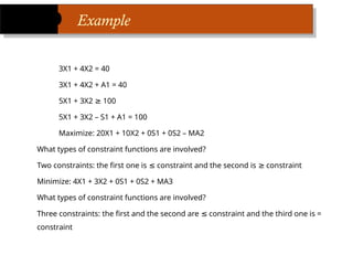
Example
3X1 + 4X2 = 40
3X1 + 4X2 + A1 = 40
5X1 + 3X2 100
≥
5X1 + 3X2 – S1 + A1 = 100
Maximize: 20X1 + 10X2 + 0S1 + 0S2 – MA2
What types of constraint functions are involved?
Two constraints: the first one is constraint and the second is constraint
≤ ≥
Minimize: 4X1 + 3X2 + 0S1 + 0S2 + MA3
What types of constraint functions are involved?
Three constraints: the first and the second are constraint and the third one is =
≤
constraint

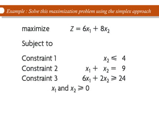
Example : Solve this maximization problem using the simplex approach

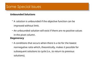
Example: Solve this Minimization Problem Using the Simplex
Method

Some Special Issues
Unbounded Solutions
– A solution is unbounded if the objective function can be
improved without limit.
– An unbounded solution will exist if there are no positive values
in the pivot column.
Degeneracy
– A conditions that occurs when there is a tie for the lowest
nonnegative ratio which, theoretically, makes it possible for
subsequent solutions to cycle (i.e., to return to previous
solutions).

Some Special Issues (cont’d)
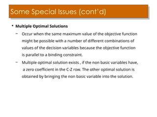
 Multiple Optimal Solutions
– Occur when the same maximum value of the objective function
might be possible with a number of different combinations of
values of the decision variables because the objective function
is parallel to a binding constraint.
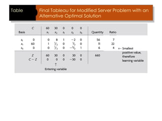
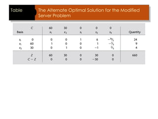
– Multiple optimal solution exists , if the non basic variables have,
a zero coefficient in the C-Z row. The other optimal solution is
obtained by bringing the non basic variable into the solution.

Table Final Tableau for Modified Server Problem with an
Alternative Optimal Solution

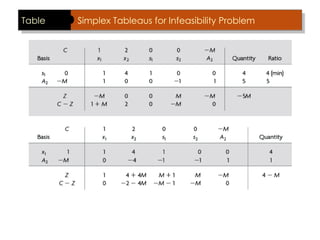
Table The Alternate Optimal Solution for the Modified
Server Problem

Some Special Issues (cont’d)
 Infeasibility
– A problem in which no combination of decision and slack/surplus
variables will simultaneously satisfy all constraints.
– Can be the result of an error in formulating a problem or it can be
because the existing set of constraints is too restrictive to permit a
solution.
– Recognized by the presence of an artificial variable in a solution that
appears optimal (i.e., a tableau in which the signs of the values in
row C – Z indicate optimality), and it has a nonzero quantity.

Table Simplex Tableaus for Infeasibility Problem

chapter 2: LINEAR PROGRAMMING FORMULATION AND SOLUTION

More Related Content

More from DejeneDay

Recently uploaded

chapter 2: LINEAR PROGRAMMING FORMULATION AND SOLUTION