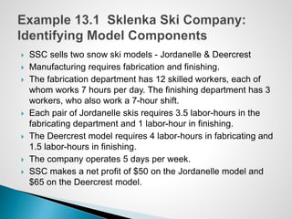
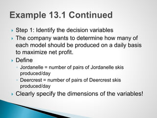
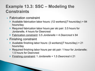
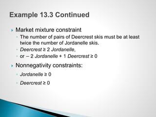
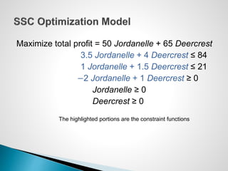
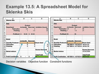
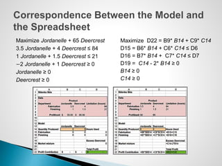
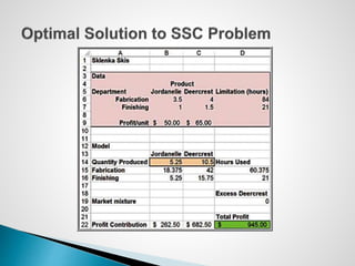
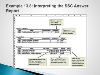
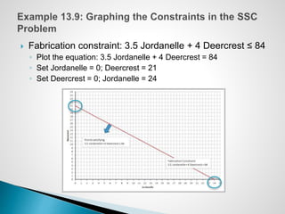
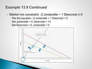
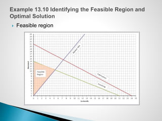
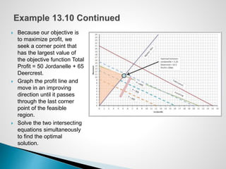
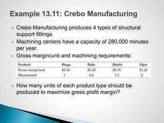
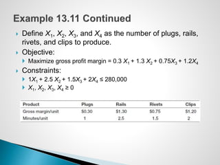
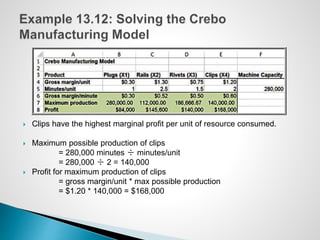
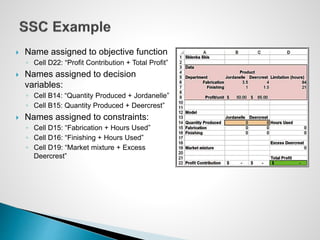
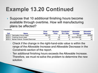
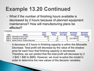
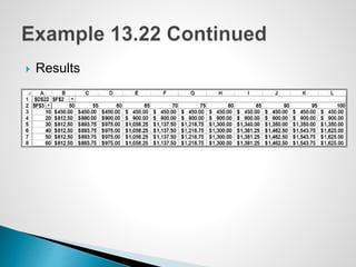
 Optimization is the process of selecting values of
decision variables that minimize or maximize
some quantity of interest.
 Optimization models have wide applicability in
operations and supply chains, finance, marketing,
and other disciplines.
 This chapter focuses only on linear optimization
models.
1. Identify the decision variables – the unknown values
that the model seeks to determine.
2. Identify the objective function – the quantity we seek
to minimize or maximize.
3. Identify all appropriate constraints – limitations,
requirements, or other restrictions that are imposed on
any solution, either from practical or technological
considerations or by management policy.
4. Write the objective function and constraints as
mathematical expressions.
 SSC sells two snow ski models - Jordanelle & Deercrest
 Manufacturing requires fabrication and finishing.
 The fabrication department has 12 skilled workers, each of
whom works 7 hours per day. The finishing department has 3
workers, who also work a 7-hour shift.
 Each pair of Jordanelle skis requires 3.5 labor-hours in the
fabricating department and 1 labor-hour in finishing.
 The Deercrest model requires 4 labor-hours in fabricating and
1.5 labor-hours in finishing.
 The company operates 5 days per week.
 SSC makes a net profit of $50 on the Jordanelle model and
$65 on the Deercrest model.
 Step 1: Identify the decision variables
 The company wants to determine how many of
each model should be produced on a daily basis
to maximize net profit.
 Define
◦ Jordanelle = number of pairs of Jordanelle skis
produced/day
◦ Deercrest = number of pairs of Deercrest skis
produced/day
 Clearly specify the dimensions of the variables!
 Step 2: Identify the objective function
 SSC wishes to maximize net profit, and we are given the
net profit figures for each type of ski.
◦ SSC makes a net profit of $50 on the Jordanelle model and $65
on the Deercrest model.
 Step 3: Identify the constraints
◦ Look for clues in the problem statement that describe limited resources
that are available, requirements that must be met, or other restrictions.
 Both the fabrication and finishing departments have limited numbers
of workers, who work only 7 hours each day; this limits the amount
of production time available in each department:
◦ Fabrication: Total labor hours used in fabrication cannot exceed the amount of
labor hours available.
◦ Finishing: Total labor hours used in finishing cannot exceed the amount of labor
hours available.
 The problem also notes that the company anticipates selling at least
twice as many Deercrest models as Jordanelle models:
◦ Number of pairs of Deercrest skis must be at leasttwice the number of parts of
Jordanelle skis.
 Negative values of the decision variables cannot occur
(“nonnegativity constraints”)
 Represent decision variables by descriptive
names, abbreviations, or subscripted letters
(X1, X2, etc.)
◦ For mathematical formulations involving many
variables, subscripted letters are often more
convenient.
◦ In spreadsheet models, we recommend using
more descriptive names to make the models and
solutions easier to understand.
 Profit per pair of skis sold:
$50 for Jordanelle skis, $65 for Deercrest skis
 Objective Function:
Maximize total profit
= 50 Jordanelle + 65 Deercrest
 Note how the dimensions verify that the
expression is correct:
◦ ($/pair of skis)(number of pairs of skis) = $.
 Constraints are expressed as algebraic inequalities or
equations, with all variables on the left side and constant
terms on the right.
 Look for key words in word statements of constraints:
◦ “Cannot exceed” translates mathematically as “≤”
◦ “At least,” would translate as “≥”
◦ “Must contain exactly,” would specify an “= ” relationship.
 All constraints in optimization models must be one of
these three forms.
 A constraint function is the left-hand side of a
constraint.
◦ E.g.: Total labor-hours used in fabrication cannot
exceed the amount of labor hours available.
 Fabrication constraint
 Available fabrication labor hours: (12 workers)(7 hours/day) = 84
hours/day
 Required fabrication labor hours per ski pair: 3.5 hours for
Jordanelle, 4 hours for Deercrest
 Fabrication constraint: 3.5 Jordanelle + 4 Deercrest ≤ 84
 Finishing constraint
 Available finishing labor hours: (3 workers)(7 hours/day) = 21
hours/day
 Required finishing labor hours per ski pair: 1 hour for Jordanelle;
1.5 hours for Deercrest
 Finishing constraint: 1 Jordanelle + 1.5 Deercrest ≤ 21
 Market mixture constraint
◦ The number of pairs of Deercrest skis must be at least
twice the number of Jordanelle skis.
◦ Deercrest ≥ 2 Jordanelle,
◦ or − 2 Jordanelle + 1 Deercrest ≥ 0
 Nonnegativity constraints:
◦ Jordanelle ≥ 0
◦ Deercrest ≥ 0
Maximize total profit = 50 Jordanelle + 65 Deercrest
3.5 Jordanelle + 4 Deercrest ≤ 84
1 Jordanelle + 1.5 Deercrest ≤ 21
−2 Jordanelle + 1 Deercrest ≥ 0
Jordanelle ≥ 0
Deercrest ≥ 0
The highlighted portions are the constraint functions
 Some examples:
 The amount of money spent on research and
development projects cannot exceed the assigned
budget of $300,000.
◦ Amount spent on research and development ≤ 300,000
 Contractual requirements specify that at least 500 units
of product must be produced.
◦ Number of units of product produced ≥ 500
 A mixture of fertilizer must contain exactly 30% nitrogen.
◦ Amount of nitrogen in mixture/total amount in mixture = 0.30
 A fertilizer mixture is made of two ingredients and must contain exactly
30% nitrogen. Ingredient X contains 20% nitrogen. Ingredient Y
contains 33% nitrogen.
 Define x = the number of pounds of X in the mixture and y = the
number of pounds of Y in the mixture
◦ Amount of nitrogen in mixture = 0.20x + 0.33y
◦ Total amount of mixture = x + y
◦ Fraction of nitrogen in mix = (0.20x + 0.33y)/(x + y)
 Since the fraction of nitrogen must be 0.30, the constraint
would be
(0.20x + 0.33y)/(x + y) = 0.30, or simplified as -0.1x - 0.03y = 0
 Note that the first version is not linear; however the simplified
constraint is linear.
 A linear optimization model (often called a
linear program, or LP) has two basic properties.
1. The objective function and all constraints are
linear functions of the decision variables.
◦ This means that each function is simply a sum of terms,
each of which is some constant multiplied by a decision
variable.
2. All variables are continuous
◦ This means that they may assume any real value
(typically, nonnegative).
 Put the objective function coefficients, constraint coefficients, and
right-hand values in a logical format in the spreadsheet.
◦ For example, you might assign the decision variables to columns and the
constraints to rows
 Define a set of cells (either rows or columns) for the values of the
decision variables.
◦ The names of the decision variables should be listed directly above the
decision variable cells.
◦ Use shading or other formatting to distinguish these cells.
 Define separate cells for the objective function and each constraint
function (the left-hand side of a constraint).
◦ Use descriptive labels directly above these cells.
Decision variables Objective function Constraint functions
Maximize Jordanelle + 65 Deercrest
3.5 Jordanelle + 4 Deercrest ≤ 84
1 Jordanelle + 1.5 Deercrest ≤ 21
−2 Jordanelle + 1 Deercrest ≥ 0
Jordanelle ≥ 0
Deercrest ≥ 0
Maximize D22 = B9* B14 + C9* C14
D15 = B6* B14 + C6* C14 ≤ D6
D16 = B7* B14 + C7* C14 ≤ D7
D19 = C14 - 2* B14 ≥ 0
B14 ≥ 0
C14 ≥ 0
 In Excel, the pairwise sum of products of terms
can easily be computed using the SUMPRODUCT
function.
◦ B9* B14 + C9*C14 = SUMPRODUCT(B9:C9,B14:C14)
 This often simplifies the model-building process,
particularly when many variables are involved.
 Several common functions in Excel can cause difficulties
when attempting to solve linear programs using Solver
because they are discontinuous (or “nonsmooth”) and do
not satisfy the conditions of a linear model.
 These include:
◦ IF
◦ MAX
◦ INT
◦ ROUND
◦ COUNT
 A feasible solution to an optimization problem is
any solution that satisfies all of the constraints.
 An optimal solution is the best of all the feasible
solutions.
 Software for determining optimal solutions
◦ Solver (“standard Solver”) is a free add-in packaged with
Excel for solving optimization problems.
◦ Premium Solver, which is a part of Analytic Solver
Platform has better functionality, accuracy, reporting, and
interface.
 Data > Analysis > Solver in the Excel ribbon
 Use the Solver Parameters dialog to define the
objective, decision variables, and constraints from
your spreadsheet model.
 Solver Parameters dialog
Objective function cell
Decision variables cells
Constraints
to enter click Add and fill in the Add
Constraint dialog:
Check box for Nonnegativity Always select “Simplex LP”
 Three reports: Answer,
Sensitivity, and Limits
◦ To add them to your Excel
workbook, click on the
ones you want and then
click OK.
 Do not check the box
Outline Reports; this is
an Excel feature that
produces the reports in
"outlined format."
 After installing Analytic Solver Platform, Premium
Solver will be found under the Add-Ins tab in the
Excel ribbon.
 Premium Solver has a different user interface than
the standard Solver.
 Solver Parameters
dialog
 First, click on Objective
and then click the Add
button. The Add
Objective dialog
appears, prompting you
for the cell reference for
the objective function
and the type of objective
(min or max).
 Next, highlight Normal
under the Variables list
and click Add; this will
bring up an Add
Variable Cells dialog.
Enter the range of the
decisions variables in
the Cell Reference field.
 Next, highlight Normal
under the Constraints
list and click the Add
button; this brings up
the Add Constraint
dialog, just like in the
standard version.
 Check this box
 Select “Standard
LP/Quadratic” for the
solving method
 Completed
Premium Solver
dialog
 The Solver Answer Report provides basic information about the
solution, including the values of the original and optimal objective
function (in the Objective Cell section) and decision variables (in the
Decision Variable Cells section).
 In the Constraints section, Cell Value refers to the value of the
constraint function using the optimal values of the decision
variables.
 A binding constraint is one for which the Cell Value is equal to the
right-hand side of the value of the constraint.
 The Status column tells whether each constraint is binding or not
binding.
 Slack refers to the difference between the left- and right-hand sides
of the constraints for the optimal solution.
 Understanding slack values
Maximize profit = 50 Jordanelle + 65 Deercrest
3.5 Jordanelle + 4 Deercrest ≤ 84 (fabrication)
1 Jordanelle + 1.5 Deercrest ≤ 21 (finishing)
−2 Jordanelle + 1 Deercrest ≥ 0 (market mix)
Jordanelle ≥ 0
Deercrest ≥ 0
Optimal solution: Jordanelle = 5.25; Deercrest = 10.5
Fabrication constraint: 3.5(5.25) + 4(10.5) = 60.375 ≤ 84
 23.625 excess fabrication hours
Finishing constraint: 1(5.25) + 1.5(10.5) = 21 ≤ 21
 No excess finishing hours
Market mix constraint: −2(5.25) + 1(10.5) = 0 ≥ 0
 Exactly twice the number of Deercrest skis as Jordanelle skis
 The set of feasible solutions is called the feasible region.
 For a problem with only two decision variables, x1 and x2, we can draw the
feasible region on a two-dimensional coordinate system by plotting the
equations corresponding to each constraint.
 Nonnegativity constraints:
 Fabrication constraint: 3.5 Jordanelle + 4 Deercrest ≤ 84
◦ Plot the equation: 3.5 Jordanelle + 4 Deercrest = 84
◦ Set Jordanelle = 0; Deercrest = 21
◦ Set Deercrest = 0; Jordanelle = 24
 Finishing constraint: 1 Jordanelle + 1.5 Deercrest ≤ 21
◦ Plot the equation: 1 Jordanelle + 1.5 Deercrest = 21
◦ Set Jordanelle = 0; Deercrest = 14
◦ Set Deercrest = 0; Jordanelle = 21
 Market mix constraint: -2 Jordanelle + 1 Deercrest ≥ 0
◦ Plot the equation: -2 Jordanelle + 1 Deercrest = 0
◦ Set Jordanelle = 5; Deercrest = 10
◦ Set Deercrest = 0; Jordanelle = 0
 Feasible region
 The points at which the constraint lines intersect along
the feasible region are called corner points.
 If an optimal solution exists, then it will occur at a corner
point.
 Because our objective is
to maximize profit, we
seek a corner point that
has the largest value of
the objective function Total
Profit = 50 Jordanelle + 65
Deercrest.
 Graph the profit line and
move in an improving
direction until it passes
through the last corner
point of the feasible
region.
 Solve the two intersecting
equations simultaneously
to find the optimal
solution.
 Solver uses a mathematical algorithm called the simplex
method, which was developed in 1947 by the late Dr.
George Dantzig.
◦ The simplex method characterizes feasible solutions algebraically
by solving systems of linear equations.
◦ It moves systematically from one corner point to another to
improve the objective function until an optimal solution is found (or
until the problem is deemed infeasible or unbounded).
◦ It is quick and efficient.
 Crebo Manufacturing produces 4 types of structural
support fittings.
 Machining centers have a capacity of 280,000 minutes
per year.
 Gross margin/unit and machining requirements:
 How many units of each product type should be
produced to maximize gross profit margin?
 Define X1, X2, X3, and X4 as the number of plugs, rails,
rivets, and clips to produce.
 Objective:
 Maximize gross profit margin = 0.3 X1 + 1.3 X2 + 0.75X3 + 1.2X4
 Constraints:
 1X1 + 2.5 X2 + 1.5X3 + 2X4 ≤ 280,000
 X1, X2, X3, X4 ≥ 0
 The simplex method evaluates the impact of constraints
in terms of their contribution to the objective function for
each variable.
 For the simple case of only one constraint, the optimal
(maximum) solution is found by simply choosing the
variable with the highest ratio of the objective coefficient
to the constraint coefficient.
 Clips have the highest marginal profit per unit of resource consumed.
 Maximum possible production of clips
= 280,000 minutes ÷ minutes/unit
= 280,000 ÷ 2 = 140,000
 Profit for maximum production of clips
= gross margin/unit * max possible production
= $1.20 * 140,000 = $168,000
 Solver assigns names to:
◦ Target cells
◦ Changing cells
◦ Constraint function cells
 Names are formed by concatenating the first cell
containing text to the:
◦ Left of the cell and
◦ Above the cell
 Name assigned to objective function
◦ Cell D22: “Profit Contribution + Total Profit”
 Names assigned to decision
variables:
◦ Cell B14: “Quantity Produced + Jordanelle”
◦ Cell B15: Quantity Produced + Deercrest”
 Names assigned to constraints:
◦ Cell D15: “Fabrication + Hours Used”
◦ Cell D16: “Finishing + Hours Used”
◦ Cell D19: “Market mixture + Excess
Deercrest”
 Unique optimal solution
◦ there is exactly one solution that will result in the maximum (or
minimum) objective.
 Alternative (multiple) optimal solutions
◦ the objective is maximized (or minimized) by more than one
combination of decision variables, all of which have the same
objective function value.
 Unbounded solution
◦ the objective can be increased or decreased without bound (i.e.,
to infinity for a maximization problem or negative infinity for a
minimization problem)
 Infeasibility
◦ no feasible solution exists
13-
 New objective function in the SSC problem:
◦ Max 50 Jordanelle + 75 Deercrest
 Remove the finishing and fabrication constraints from the Sklenka
Ski problem.
 Solver message:
 Suppose, by mistake, the modeler in the Sklenka Ski problem used
a ≥ sign in the fabrication constraint (instead of ≤):
 Models should be used to provide insight for
making better decisions.
◦ What might happen should the model assumptions
change or when the data used in the model are
uncertain?
◦ With Solver, answers to such questions can easily be
found by simply changing the data and re-solving the
model.
 Four questions are posed by the managers of
Sklenka Ski company:
1. If the Jordanelle ski’s profit increased $10/pair,
how would the optimal solution change?
2. If the Jordanelle ski’s profit decreased $10/pair,
how would the optimal solution change?
3. If 10 additional finishing hours were available,
how would manufacturing plans be affected?
4. If 2 fewer finishing hours were available, how
would manufacturing plans be affected?
 Summary of What-If scenarios:
 The Sensitivity Report allows us to understand how
◦ the optimal objective value and optimal decision variables
are affected by changes in the objective function
coefficients,
◦ the impact of forced changes in certain decision variables,
or
◦ the impact of changes in the constraint resource limitations
or requirements.
 The Sensitivity Report information applies to changes in
only one of the model parameters at a time; all others
are assumed to remain at their original values.
Reduced Cost: How much the objective function coefficient needs to be
reduced for a nonnegative variable that is zero in the optimal solution to
become positive. If a variable is positive in the optimal solution, its reduced
cost is zero.
If the objective coefficient of any one variable that has positive value in the
current solution changes but stays within the range specified by the Allowable
Increase and Allowable Decrease, the optimal decision variables will stay the
same; however, the objective function value will change.
 Sensitivity report for the Sklenka Ski model after
changing the profit on Jordanelle skis from $50 to $40
Shadow Price - how much the objective function will change as the
right hand side of a constraint is increased by 1.
Whenever a constraint has positive slack, the shadow price is zero.
When a constraint involves a limited resource, the shadow price
represents the economic value of having an additional unit of that
resource.
 Shows the upper and lower limits that each
decision variable can assume while satisfying all
constraints and holding the other variables
constant.
 If a change in an objective function coefficient remains
within the Allowable Increase and Allowable Decrease
ranges in the Decision Variable Cells section of the
report, then the optimal values of the decision variables
will not change. However, you must recalculate the value
of the objective function using the new value of the
coefficient.
 If a change in an objective function coefficient exceeds
the Allowable Increase or Allowable Decrease limits in
the Decision Variable Cells section of the report, then
you must re-solve the model to find the new optimal
values.
 If a change in the right-hand side of a constraint remains
within the Allowable Increase and Allowable Decrease ranges
in the Constraints section of the report, then the shadow price
allows you to predict how the objective function value will
change. Multiply the change in the right-hand side (positive if
an increase, negative if a decrease) by the value of the
shadow price. However, you must re-solve the model to find
the new values of the decision variables.
 If a change in the right-hand side of a constraint exceeds the
Allowable Increase or Allowable Decrease limits in the
Constraints section of the report, then you cannot predict how
the objective function value will change using the shadow
price. You must re-solve the problem to find the new solution.
 Suppose that the unit profit on Jordanelle skis is increased by $10.
How will the optimal solution change? What is the best product mix?
◦ Is the increase in the objective function coefficient is within the range of
the Allowable Increase and Allowable Decrease in the Decision Variable
Cells portion of the report?
◦ Because $10 is less than the Allowable Increase of infinity, we can safely
conclude that the optimal quantities of the decision variables will not
change.
◦ However, because the objective function changed, we need to compute
the new value of the total profit: 5.25($60) + 10.5($65) = $997.50.
 Suppose that the unit profit on Jordanelle skis is
decreased by $10 because of higher material costs. How
will the optimal solution change? What is the best
product mix?
◦ The change in the unit profit exceeds the Allowable Decrease
($6.67). We can conclude that the optimal values of the decision
variables will change, although we must re-solve the problem to
determine what the new values would be.
 Suppose that 10 additional finishing hours become
available through overtime. How will manufacturing
plans be affected?
◦ Check if the change in the right-hand-side value is within the
range of the Allowable Increase and Allowable Decrease in the
Constraints section of the report.
◦ Ten additional finishing hours exceeds the Allowable Increase.
Therefore, we must re-solve the problem to determine the new
solution.
 What if the number of finishing hours available is
decreased by 2 hours because of planned equipment
maintenance? How will manufacturing plans be
affected?
◦ A decrease of 2 hours in finishing capacity is within the Allowable
Decrease. Total profit will decrease by the value of the shadow
price for each hour that finishing capacity is decreased.
Therefore, we can predict that the total profit will decrease by 2
×$45 = $90 to $855. However, we must re-solve the model in
order to determine the new values of the decision variables.
 Solver can be used to perform sensitivity analysis
by either:
 Examining the sensitivity reports or
 Changing data in the model and re-solving it
 Analytic Solver Platform offers an alternative
approach to sensitivity analysis called parameter
analysis, which allows you to run multiple
optimizations while varying model parameters
within predefined ranges.
 Investigate the impact of
changing finishing hour
capacity over a range from
10 to 60.
◦ Choose an empty cell in the
spreadsheet (e.g., F3)
◦ From Analytic Solver Platform
ribbon, click Parameters button
and choose Optimization.
◦ Define range in Function
Arguments dialog.
◦ Replace the value in cell D7 by
=F3
 From the Reports button in the
Analysis group in the Analytic
Solver Platform ribbon, select
Optimization Reports and then
Parameter Analysis
 Move decision variable and
objective function cells to the right
Result Cells pane, and move the
parameter cell F3 to the right
Parameters pane.
 In the drop-down box, select Vary
All Selected Parameters
Simultaneously.
 Set Major Axis Points to number
of parameter values to test.
 Parameter analysis results
◦ Reformat the results to make them easier to understand.
For example, name the columns with descriptive labels
instead of cell references; use charts to visualize the
results.
 Suppose that we wish to examine the effect on the
optimal profit of changing both the Fabrication and
Finishing hour limitations, similar to a two-way
data table.
 Follow the procedure in Example 13.21 to define
the parameter for the Finishing limitation.
◦ In the Function Arguments dialog, set the range for the
Fabrication limitation between 50 and 100.
 In the Multiple Optimizations
Report dialog, choose both
parameter cells F2 and F3;
however, we can only choose
one result cell. In this case,
choose $D$22, which represents
the objective function value.
 In the drop-down box, select Vary
Two Selected Parameters
Independently.
 Results

Evans_Analytics2e_ppt_13.pptxbbbbbbbbbbb

  • 2.
     Optimization isthe process of selecting values of decision variables that minimize or maximize some quantity of interest.  Optimization models have wide applicability in operations and supply chains, finance, marketing, and other disciplines.  This chapter focuses only on linear optimization models.
  • 3.
    1. Identify thedecision variables – the unknown values that the model seeks to determine. 2. Identify the objective function – the quantity we seek to minimize or maximize. 3. Identify all appropriate constraints – limitations, requirements, or other restrictions that are imposed on any solution, either from practical or technological considerations or by management policy. 4. Write the objective function and constraints as mathematical expressions.
  • 4.
     SSC sellstwo snow ski models - Jordanelle & Deercrest  Manufacturing requires fabrication and finishing.  The fabrication department has 12 skilled workers, each of whom works 7 hours per day. The finishing department has 3 workers, who also work a 7-hour shift.  Each pair of Jordanelle skis requires 3.5 labor-hours in the fabricating department and 1 labor-hour in finishing.  The Deercrest model requires 4 labor-hours in fabricating and 1.5 labor-hours in finishing.  The company operates 5 days per week.  SSC makes a net profit of $50 on the Jordanelle model and $65 on the Deercrest model.
  • 5.
     Step 1:Identify the decision variables  The company wants to determine how many of each model should be produced on a daily basis to maximize net profit.  Define ◦ Jordanelle = number of pairs of Jordanelle skis produced/day ◦ Deercrest = number of pairs of Deercrest skis produced/day  Clearly specify the dimensions of the variables!
  • 6.
     Step 2:Identify the objective function  SSC wishes to maximize net profit, and we are given the net profit figures for each type of ski. ◦ SSC makes a net profit of $50 on the Jordanelle model and $65 on the Deercrest model.
  • 7.
     Step 3:Identify the constraints ◦ Look for clues in the problem statement that describe limited resources that are available, requirements that must be met, or other restrictions.  Both the fabrication and finishing departments have limited numbers of workers, who work only 7 hours each day; this limits the amount of production time available in each department: ◦ Fabrication: Total labor hours used in fabrication cannot exceed the amount of labor hours available. ◦ Finishing: Total labor hours used in finishing cannot exceed the amount of labor hours available.  The problem also notes that the company anticipates selling at least twice as many Deercrest models as Jordanelle models: ◦ Number of pairs of Deercrest skis must be at leasttwice the number of parts of Jordanelle skis.  Negative values of the decision variables cannot occur (“nonnegativity constraints”)
  • 8.
     Represent decisionvariables by descriptive names, abbreviations, or subscripted letters (X1, X2, etc.) ◦ For mathematical formulations involving many variables, subscripted letters are often more convenient. ◦ In spreadsheet models, we recommend using more descriptive names to make the models and solutions easier to understand.
  • 9.
     Profit perpair of skis sold: $50 for Jordanelle skis, $65 for Deercrest skis  Objective Function: Maximize total profit = 50 Jordanelle + 65 Deercrest  Note how the dimensions verify that the expression is correct: ◦ ($/pair of skis)(number of pairs of skis) = $.
  • 10.
     Constraints areexpressed as algebraic inequalities or equations, with all variables on the left side and constant terms on the right.  Look for key words in word statements of constraints: ◦ “Cannot exceed” translates mathematically as “≤” ◦ “At least,” would translate as “≥” ◦ “Must contain exactly,” would specify an “= ” relationship.  All constraints in optimization models must be one of these three forms.
  • 11.
     A constraintfunction is the left-hand side of a constraint. ◦ E.g.: Total labor-hours used in fabrication cannot exceed the amount of labor hours available.
  • 12.
     Fabrication constraint Available fabrication labor hours: (12 workers)(7 hours/day) = 84 hours/day  Required fabrication labor hours per ski pair: 3.5 hours for Jordanelle, 4 hours for Deercrest  Fabrication constraint: 3.5 Jordanelle + 4 Deercrest ≤ 84  Finishing constraint  Available finishing labor hours: (3 workers)(7 hours/day) = 21 hours/day  Required finishing labor hours per ski pair: 1 hour for Jordanelle; 1.5 hours for Deercrest  Finishing constraint: 1 Jordanelle + 1.5 Deercrest ≤ 21
  • 13.
     Market mixtureconstraint ◦ The number of pairs of Deercrest skis must be at least twice the number of Jordanelle skis. ◦ Deercrest ≥ 2 Jordanelle, ◦ or − 2 Jordanelle + 1 Deercrest ≥ 0  Nonnegativity constraints: ◦ Jordanelle ≥ 0 ◦ Deercrest ≥ 0
  • 14.
    Maximize total profit= 50 Jordanelle + 65 Deercrest 3.5 Jordanelle + 4 Deercrest ≤ 84 1 Jordanelle + 1.5 Deercrest ≤ 21 −2 Jordanelle + 1 Deercrest ≥ 0 Jordanelle ≥ 0 Deercrest ≥ 0 The highlighted portions are the constraint functions
  • 15.
     Some examples: The amount of money spent on research and development projects cannot exceed the assigned budget of $300,000. ◦ Amount spent on research and development ≤ 300,000  Contractual requirements specify that at least 500 units of product must be produced. ◦ Number of units of product produced ≥ 500  A mixture of fertilizer must contain exactly 30% nitrogen. ◦ Amount of nitrogen in mixture/total amount in mixture = 0.30
  • 16.
     A fertilizermixture is made of two ingredients and must contain exactly 30% nitrogen. Ingredient X contains 20% nitrogen. Ingredient Y contains 33% nitrogen.  Define x = the number of pounds of X in the mixture and y = the number of pounds of Y in the mixture ◦ Amount of nitrogen in mixture = 0.20x + 0.33y ◦ Total amount of mixture = x + y ◦ Fraction of nitrogen in mix = (0.20x + 0.33y)/(x + y)  Since the fraction of nitrogen must be 0.30, the constraint would be (0.20x + 0.33y)/(x + y) = 0.30, or simplified as -0.1x - 0.03y = 0  Note that the first version is not linear; however the simplified constraint is linear.
  • 17.
     A linearoptimization model (often called a linear program, or LP) has two basic properties. 1. The objective function and all constraints are linear functions of the decision variables. ◦ This means that each function is simply a sum of terms, each of which is some constant multiplied by a decision variable. 2. All variables are continuous ◦ This means that they may assume any real value (typically, nonnegative).
  • 18.
     Put theobjective function coefficients, constraint coefficients, and right-hand values in a logical format in the spreadsheet. ◦ For example, you might assign the decision variables to columns and the constraints to rows  Define a set of cells (either rows or columns) for the values of the decision variables. ◦ The names of the decision variables should be listed directly above the decision variable cells. ◦ Use shading or other formatting to distinguish these cells.  Define separate cells for the objective function and each constraint function (the left-hand side of a constraint). ◦ Use descriptive labels directly above these cells.
  • 19.
    Decision variables Objectivefunction Constraint functions
  • 20.
    Maximize Jordanelle +65 Deercrest 3.5 Jordanelle + 4 Deercrest ≤ 84 1 Jordanelle + 1.5 Deercrest ≤ 21 −2 Jordanelle + 1 Deercrest ≥ 0 Jordanelle ≥ 0 Deercrest ≥ 0 Maximize D22 = B9* B14 + C9* C14 D15 = B6* B14 + C6* C14 ≤ D6 D16 = B7* B14 + C7* C14 ≤ D7 D19 = C14 - 2* B14 ≥ 0 B14 ≥ 0 C14 ≥ 0
  • 21.
     In Excel,the pairwise sum of products of terms can easily be computed using the SUMPRODUCT function. ◦ B9* B14 + C9*C14 = SUMPRODUCT(B9:C9,B14:C14)  This often simplifies the model-building process, particularly when many variables are involved.
  • 22.
     Several commonfunctions in Excel can cause difficulties when attempting to solve linear programs using Solver because they are discontinuous (or “nonsmooth”) and do not satisfy the conditions of a linear model.  These include: ◦ IF ◦ MAX ◦ INT ◦ ROUND ◦ COUNT
  • 23.
     A feasiblesolution to an optimization problem is any solution that satisfies all of the constraints.  An optimal solution is the best of all the feasible solutions.  Software for determining optimal solutions ◦ Solver (“standard Solver”) is a free add-in packaged with Excel for solving optimization problems. ◦ Premium Solver, which is a part of Analytic Solver Platform has better functionality, accuracy, reporting, and interface.
  • 24.
     Data >Analysis > Solver in the Excel ribbon  Use the Solver Parameters dialog to define the objective, decision variables, and constraints from your spreadsheet model.
  • 25.
     Solver Parametersdialog Objective function cell Decision variables cells Constraints to enter click Add and fill in the Add Constraint dialog: Check box for Nonnegativity Always select “Simplex LP”
  • 26.
     Three reports:Answer, Sensitivity, and Limits ◦ To add them to your Excel workbook, click on the ones you want and then click OK.  Do not check the box Outline Reports; this is an Excel feature that produces the reports in "outlined format."
  • 28.
     After installingAnalytic Solver Platform, Premium Solver will be found under the Add-Ins tab in the Excel ribbon.  Premium Solver has a different user interface than the standard Solver.
  • 29.
     Solver Parameters dialog First, click on Objective and then click the Add button. The Add Objective dialog appears, prompting you for the cell reference for the objective function and the type of objective (min or max).
  • 30.
     Next, highlightNormal under the Variables list and click Add; this will bring up an Add Variable Cells dialog. Enter the range of the decisions variables in the Cell Reference field.
  • 31.
     Next, highlightNormal under the Constraints list and click the Add button; this brings up the Add Constraint dialog, just like in the standard version.
  • 32.
     Check thisbox  Select “Standard LP/Quadratic” for the solving method
  • 33.
  • 34.
     The SolverAnswer Report provides basic information about the solution, including the values of the original and optimal objective function (in the Objective Cell section) and decision variables (in the Decision Variable Cells section).  In the Constraints section, Cell Value refers to the value of the constraint function using the optimal values of the decision variables.  A binding constraint is one for which the Cell Value is equal to the right-hand side of the value of the constraint.  The Status column tells whether each constraint is binding or not binding.  Slack refers to the difference between the left- and right-hand sides of the constraints for the optimal solution.
  • 36.
     Understanding slackvalues Maximize profit = 50 Jordanelle + 65 Deercrest 3.5 Jordanelle + 4 Deercrest ≤ 84 (fabrication) 1 Jordanelle + 1.5 Deercrest ≤ 21 (finishing) −2 Jordanelle + 1 Deercrest ≥ 0 (market mix) Jordanelle ≥ 0 Deercrest ≥ 0 Optimal solution: Jordanelle = 5.25; Deercrest = 10.5 Fabrication constraint: 3.5(5.25) + 4(10.5) = 60.375 ≤ 84  23.625 excess fabrication hours Finishing constraint: 1(5.25) + 1.5(10.5) = 21 ≤ 21  No excess finishing hours Market mix constraint: −2(5.25) + 1(10.5) = 0 ≥ 0  Exactly twice the number of Deercrest skis as Jordanelle skis
  • 37.
     The setof feasible solutions is called the feasible region.  For a problem with only two decision variables, x1 and x2, we can draw the feasible region on a two-dimensional coordinate system by plotting the equations corresponding to each constraint.  Nonnegativity constraints:
  • 38.
     Fabrication constraint:3.5 Jordanelle + 4 Deercrest ≤ 84 ◦ Plot the equation: 3.5 Jordanelle + 4 Deercrest = 84 ◦ Set Jordanelle = 0; Deercrest = 21 ◦ Set Deercrest = 0; Jordanelle = 24
  • 39.
     Finishing constraint:1 Jordanelle + 1.5 Deercrest ≤ 21 ◦ Plot the equation: 1 Jordanelle + 1.5 Deercrest = 21 ◦ Set Jordanelle = 0; Deercrest = 14 ◦ Set Deercrest = 0; Jordanelle = 21
  • 40.
     Market mixconstraint: -2 Jordanelle + 1 Deercrest ≥ 0 ◦ Plot the equation: -2 Jordanelle + 1 Deercrest = 0 ◦ Set Jordanelle = 5; Deercrest = 10 ◦ Set Deercrest = 0; Jordanelle = 0
  • 41.
  • 42.
     The pointsat which the constraint lines intersect along the feasible region are called corner points.  If an optimal solution exists, then it will occur at a corner point.
  • 43.
     Because ourobjective is to maximize profit, we seek a corner point that has the largest value of the objective function Total Profit = 50 Jordanelle + 65 Deercrest.  Graph the profit line and move in an improving direction until it passes through the last corner point of the feasible region.  Solve the two intersecting equations simultaneously to find the optimal solution.
  • 44.
     Solver usesa mathematical algorithm called the simplex method, which was developed in 1947 by the late Dr. George Dantzig. ◦ The simplex method characterizes feasible solutions algebraically by solving systems of linear equations. ◦ It moves systematically from one corner point to another to improve the objective function until an optimal solution is found (or until the problem is deemed infeasible or unbounded). ◦ It is quick and efficient.
  • 45.
     Crebo Manufacturingproduces 4 types of structural support fittings.  Machining centers have a capacity of 280,000 minutes per year.  Gross margin/unit and machining requirements:  How many units of each product type should be produced to maximize gross profit margin?
  • 46.
     Define X1,X2, X3, and X4 as the number of plugs, rails, rivets, and clips to produce.  Objective:  Maximize gross profit margin = 0.3 X1 + 1.3 X2 + 0.75X3 + 1.2X4  Constraints:  1X1 + 2.5 X2 + 1.5X3 + 2X4 ≤ 280,000  X1, X2, X3, X4 ≥ 0
  • 47.
     The simplexmethod evaluates the impact of constraints in terms of their contribution to the objective function for each variable.  For the simple case of only one constraint, the optimal (maximum) solution is found by simply choosing the variable with the highest ratio of the objective coefficient to the constraint coefficient.
  • 48.
     Clips havethe highest marginal profit per unit of resource consumed.  Maximum possible production of clips = 280,000 minutes ÷ minutes/unit = 280,000 ÷ 2 = 140,000  Profit for maximum production of clips = gross margin/unit * max possible production = $1.20 * 140,000 = $168,000
  • 49.
     Solver assignsnames to: ◦ Target cells ◦ Changing cells ◦ Constraint function cells  Names are formed by concatenating the first cell containing text to the: ◦ Left of the cell and ◦ Above the cell
  • 50.
     Name assignedto objective function ◦ Cell D22: “Profit Contribution + Total Profit”  Names assigned to decision variables: ◦ Cell B14: “Quantity Produced + Jordanelle” ◦ Cell B15: Quantity Produced + Deercrest”  Names assigned to constraints: ◦ Cell D15: “Fabrication + Hours Used” ◦ Cell D16: “Finishing + Hours Used” ◦ Cell D19: “Market mixture + Excess Deercrest”
  • 51.
     Unique optimalsolution ◦ there is exactly one solution that will result in the maximum (or minimum) objective.  Alternative (multiple) optimal solutions ◦ the objective is maximized (or minimized) by more than one combination of decision variables, all of which have the same objective function value.  Unbounded solution ◦ the objective can be increased or decreased without bound (i.e., to infinity for a maximization problem or negative infinity for a minimization problem)  Infeasibility ◦ no feasible solution exists
  • 52.
    13-  New objectivefunction in the SSC problem: ◦ Max 50 Jordanelle + 75 Deercrest
  • 53.
     Remove thefinishing and fabrication constraints from the Sklenka Ski problem.  Solver message:
  • 54.
     Suppose, bymistake, the modeler in the Sklenka Ski problem used a ≥ sign in the fabrication constraint (instead of ≤):
  • 55.
     Models shouldbe used to provide insight for making better decisions. ◦ What might happen should the model assumptions change or when the data used in the model are uncertain? ◦ With Solver, answers to such questions can easily be found by simply changing the data and re-solving the model.
  • 56.
     Four questionsare posed by the managers of Sklenka Ski company: 1. If the Jordanelle ski’s profit increased $10/pair, how would the optimal solution change? 2. If the Jordanelle ski’s profit decreased $10/pair, how would the optimal solution change? 3. If 10 additional finishing hours were available, how would manufacturing plans be affected? 4. If 2 fewer finishing hours were available, how would manufacturing plans be affected?
  • 57.
     Summary ofWhat-If scenarios:
  • 58.
     The SensitivityReport allows us to understand how ◦ the optimal objective value and optimal decision variables are affected by changes in the objective function coefficients, ◦ the impact of forced changes in certain decision variables, or ◦ the impact of changes in the constraint resource limitations or requirements.  The Sensitivity Report information applies to changes in only one of the model parameters at a time; all others are assumed to remain at their original values.
  • 60.
    Reduced Cost: Howmuch the objective function coefficient needs to be reduced for a nonnegative variable that is zero in the optimal solution to become positive. If a variable is positive in the optimal solution, its reduced cost is zero. If the objective coefficient of any one variable that has positive value in the current solution changes but stays within the range specified by the Allowable Increase and Allowable Decrease, the optimal decision variables will stay the same; however, the objective function value will change.
  • 61.
     Sensitivity reportfor the Sklenka Ski model after changing the profit on Jordanelle skis from $50 to $40
  • 62.
    Shadow Price -how much the objective function will change as the right hand side of a constraint is increased by 1. Whenever a constraint has positive slack, the shadow price is zero. When a constraint involves a limited resource, the shadow price represents the economic value of having an additional unit of that resource.
  • 63.
     Shows theupper and lower limits that each decision variable can assume while satisfying all constraints and holding the other variables constant.
  • 64.
     If achange in an objective function coefficient remains within the Allowable Increase and Allowable Decrease ranges in the Decision Variable Cells section of the report, then the optimal values of the decision variables will not change. However, you must recalculate the value of the objective function using the new value of the coefficient.  If a change in an objective function coefficient exceeds the Allowable Increase or Allowable Decrease limits in the Decision Variable Cells section of the report, then you must re-solve the model to find the new optimal values.
  • 65.
     If achange in the right-hand side of a constraint remains within the Allowable Increase and Allowable Decrease ranges in the Constraints section of the report, then the shadow price allows you to predict how the objective function value will change. Multiply the change in the right-hand side (positive if an increase, negative if a decrease) by the value of the shadow price. However, you must re-solve the model to find the new values of the decision variables.  If a change in the right-hand side of a constraint exceeds the Allowable Increase or Allowable Decrease limits in the Constraints section of the report, then you cannot predict how the objective function value will change using the shadow price. You must re-solve the problem to find the new solution.
  • 66.
     Suppose thatthe unit profit on Jordanelle skis is increased by $10. How will the optimal solution change? What is the best product mix? ◦ Is the increase in the objective function coefficient is within the range of the Allowable Increase and Allowable Decrease in the Decision Variable Cells portion of the report? ◦ Because $10 is less than the Allowable Increase of infinity, we can safely conclude that the optimal quantities of the decision variables will not change. ◦ However, because the objective function changed, we need to compute the new value of the total profit: 5.25($60) + 10.5($65) = $997.50.
  • 67.
     Suppose thatthe unit profit on Jordanelle skis is decreased by $10 because of higher material costs. How will the optimal solution change? What is the best product mix? ◦ The change in the unit profit exceeds the Allowable Decrease ($6.67). We can conclude that the optimal values of the decision variables will change, although we must re-solve the problem to determine what the new values would be.
  • 68.
     Suppose that10 additional finishing hours become available through overtime. How will manufacturing plans be affected? ◦ Check if the change in the right-hand-side value is within the range of the Allowable Increase and Allowable Decrease in the Constraints section of the report. ◦ Ten additional finishing hours exceeds the Allowable Increase. Therefore, we must re-solve the problem to determine the new solution.
  • 69.
     What ifthe number of finishing hours available is decreased by 2 hours because of planned equipment maintenance? How will manufacturing plans be affected? ◦ A decrease of 2 hours in finishing capacity is within the Allowable Decrease. Total profit will decrease by the value of the shadow price for each hour that finishing capacity is decreased. Therefore, we can predict that the total profit will decrease by 2 ×$45 = $90 to $855. However, we must re-solve the model in order to determine the new values of the decision variables.
  • 70.
     Solver canbe used to perform sensitivity analysis by either:  Examining the sensitivity reports or  Changing data in the model and re-solving it  Analytic Solver Platform offers an alternative approach to sensitivity analysis called parameter analysis, which allows you to run multiple optimizations while varying model parameters within predefined ranges.
  • 71.
     Investigate theimpact of changing finishing hour capacity over a range from 10 to 60. ◦ Choose an empty cell in the spreadsheet (e.g., F3) ◦ From Analytic Solver Platform ribbon, click Parameters button and choose Optimization. ◦ Define range in Function Arguments dialog. ◦ Replace the value in cell D7 by =F3
  • 72.
     From theReports button in the Analysis group in the Analytic Solver Platform ribbon, select Optimization Reports and then Parameter Analysis  Move decision variable and objective function cells to the right Result Cells pane, and move the parameter cell F3 to the right Parameters pane.  In the drop-down box, select Vary All Selected Parameters Simultaneously.  Set Major Axis Points to number of parameter values to test.
  • 73.
     Parameter analysisresults ◦ Reformat the results to make them easier to understand. For example, name the columns with descriptive labels instead of cell references; use charts to visualize the results.
  • 74.
     Suppose thatwe wish to examine the effect on the optimal profit of changing both the Fabrication and Finishing hour limitations, similar to a two-way data table.  Follow the procedure in Example 13.21 to define the parameter for the Finishing limitation. ◦ In the Function Arguments dialog, set the range for the Fabrication limitation between 50 and 100.
  • 75.
     In theMultiple Optimizations Report dialog, choose both parameter cells F2 and F3; however, we can only choose one result cell. In this case, choose $D$22, which represents the objective function value.  In the drop-down box, select Vary Two Selected Parameters Independently.
  • 76.