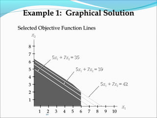
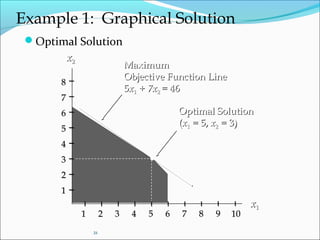
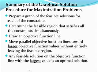
2. CHAPTER TWO
RESOURCE OPTIMIZATION
Optimization Definition:
Optimization is a process of finding the "best“(optimal)
solution to a problem
What do we mean by the "best"?
cost, performance, aesthetics, social or individual "well-
being", etc.
The terminology ‘best’ solution implies that there is more than
one solution and the solutions are not of equal value.
Optimization selects the "best" decision from a
constrained situation.
• Optimization is the process of adjusting the inputs to or
characteristics of advice, mathematical process, or experiment
to find the minimum or maximum output or result. 2
3. 2. RESOURCE OPTIMIZATION
Optimizing Methods
The methods to find an optimal solution to the
constrained resource scheduling problem fall into two
categories:
Mathematical programming
Enumeration
Mathematical programming can be thought of as
liner programming (LP) for the most part
Linear programming is usually not feasible for
reasonably large projects where there may be a
dozen resources and thousands of activities
3
4. RESOURCE OPTIMIZATION Cont….
In the late 1960s and early 1970s, limited
enumeration techniques were applied to the
constrained resource problem
Tree search, and branch and bound methods
were devised to handle up to five resources and
200 activities
But we will Discuss on Linear Programming and
Simplex algorism in this section
4
5. RESOURCE OPTIMIZATION Cont….
Linear Programming (LP)
Linear means a fixed, definable relationship between the
variables in the problem to be solved.
Programming refers to the orderly process by which this
type of problem is solved.
Their fore Linear programming is:-
A mathematical technique to help plan and make decisions
relative to the trade-offs necessary to allocate resources.
Will find the minimum or maximum value of the objective.
As its name implies, the linear programming model consists
of linear objectives and linear constraints, which means that
the variables in a model have a proportionate relationship.
Linear programming is a widely used mathematical modeling
technique to determine the optimum allocation of scarce
resources among competing demands. 5
7. Linear Programming (LP)----Cont…..
Essentials of a Linear Programming model
For a given problem situation, there are certain
essential conditions that need to be solved by using
Linear Programming.
1. Limited resources: limited number of labour, material
equipment and finance.
2.Objective: refers to the aim to optimize (maximize
the profits or minimize the costs).
3. Linearity: increase in labour input will have a
proportionate increase in output.
7
8. Linear Programming (LP)----Cont…..
The linear model consists of the following components:
A set of decision variables
An objective function
A set of constraints
1. Decision Variables
are physical quantities controlled by the decision maker
and represented by mathematical symbols. For example,
the decision variable xj can represent the number of
pounds of product j that a company will produce during
some month. Decision variables take on any of a set of
possible values
8
9. Linear Programming (LP)----Cont…..
2. Objective function
defines the criterion for evaluating the solution. It is
a mathematical function of the decision variables
that converts a solution into a numerical
evaluation of that solution. For example, the
objective function may measure the profit or cost
that occurs as a function of the amounts of various
products produced. The objective function also
specifies a direction of optimization, either to
maximize or minimize. An optimal solution for the
model is the best solution as measured by that
criterion.
9
10. Linear Programming (LP)----Cont…..
3. Constraints are a set of functional equalities or
inequalities that represent physical, economic,
technological, legal, ethical, or other restrictions on what
numerical values can be assigned to the decision variables.
For example, constraints might ensure that no more input is
used than is available. Constraints can be definitional,
defining the number of employees at the start of a period t +
1 as equal to the number of employees at the start of period t,
plus those added during period t minus those leaving the
organization during period t. In constrained optimization
models we find values for the
The three methods of solving LP:
1. Graphical method
2. Algebraic method
3. Simplex method 10
11. Linear Programming (LP) Problem
The maximization or minimization of some quantity is the
objective in all linear programming problems.
All LP problems have constraints that limit the degree to
which the objective can be pursued.
A feasible solution satisfies all the problem's constraints.
An optimal solution is a feasible solution that results in
the largest possible objective function value when
maximizing (or smallest when minimizing).
A graphical solution method can be used to solve a linear
program with two variables.
11
12. Linear Programming (LP) Problem
If both the objective function and the constraints are
linear, the problem is referred to as a linear
programming problem.
Linear functions are functions in which each variable
appears in a separate term raised to the first power
and is multiplied by a constant (which could be 0).
Linear constraints are linear functions that are
restricted to be "less than or equal to", "equal to", or
"greater than or equal to" a constant.
12
13. Problem Formulation
Problem formulation or modeling is the process of
translating a verbal statement of a problem into a
mathematical statement.
Formulating models is an art that can only be
mastered with practice and experience.
Every LP problems has some unique features, but
most problems also have common features.
General guidelines for LP model formulation are
illustrated on the slides that follow.
13
14. 14
Example 1: A Simple Maximization Problem
Max 5Max 5xx11 + 7+ 7xx22
s.t.s.t. xx11 << 66
22xx11 + 3+ 3xx22 << 1919
xx11 ++ xx22 << 88
xx11 >> 0 and0 and xx22 >> 00
ObjectiveObjective
FunctionFunction
““Regular”Regular”
ConstraintsConstraints
Non-negativityNon-negativity
ConstraintsConstraints
15. 15
Example 1: Graphical Solution
First Constraint Graphed
xx22
xx11
xx11 = 6= 6
(6, 0)(6, 0)
88
77
66
55
44
33
22
11
11 22 33 44 55 66 77 88 9 109 10
Shaded regionShaded region
contains allcontains all
feasible pointsfeasible points
for this constraintfor this constraint
16. 16
Example 1: Graphical Solution
Second Constraint Graphed
22xx11 + 3+ 3xx22=19=19
xx22
xx11
(0, 6,(0, 6,1/31/3))
(9(9 1/21/2,, 0)0)
88
77
66
55
44
33
22
11
11 22 33 44 55 66 77 88 9 109 10
ShadedShaded
region containsregion contains
all feasible pointsall feasible points
for this constraintfor this constraint
17. 17
Example 1: Graphical Solution
Third Constraint Graphed
xx22
xx11
xx11 ++ xx22 = 8= 8
(0, 8)(0, 8)
(8, 0)(8, 0)
88
77
66
55
44
33
22
11
11 22 33 44 55 66 77 88 9 109 10
ShadedShaded
region containsregion contains
all feasible pointsall feasible points
for this constraintfor this constraint
22. 22
Summary of the Graphical Solution
Procedure for Maximization Problems
Prepare a graph of the feasible solutions for
each of the constraints.
Determine the feasible region that satisfies all
the constraints simultaneously.
Draw an objective function line.
Move parallel objective function lines toward
larger objective function values without entirely
leaving the feasible region.
Any feasible solution on the objective function
line with the largest value is an optimal solution.