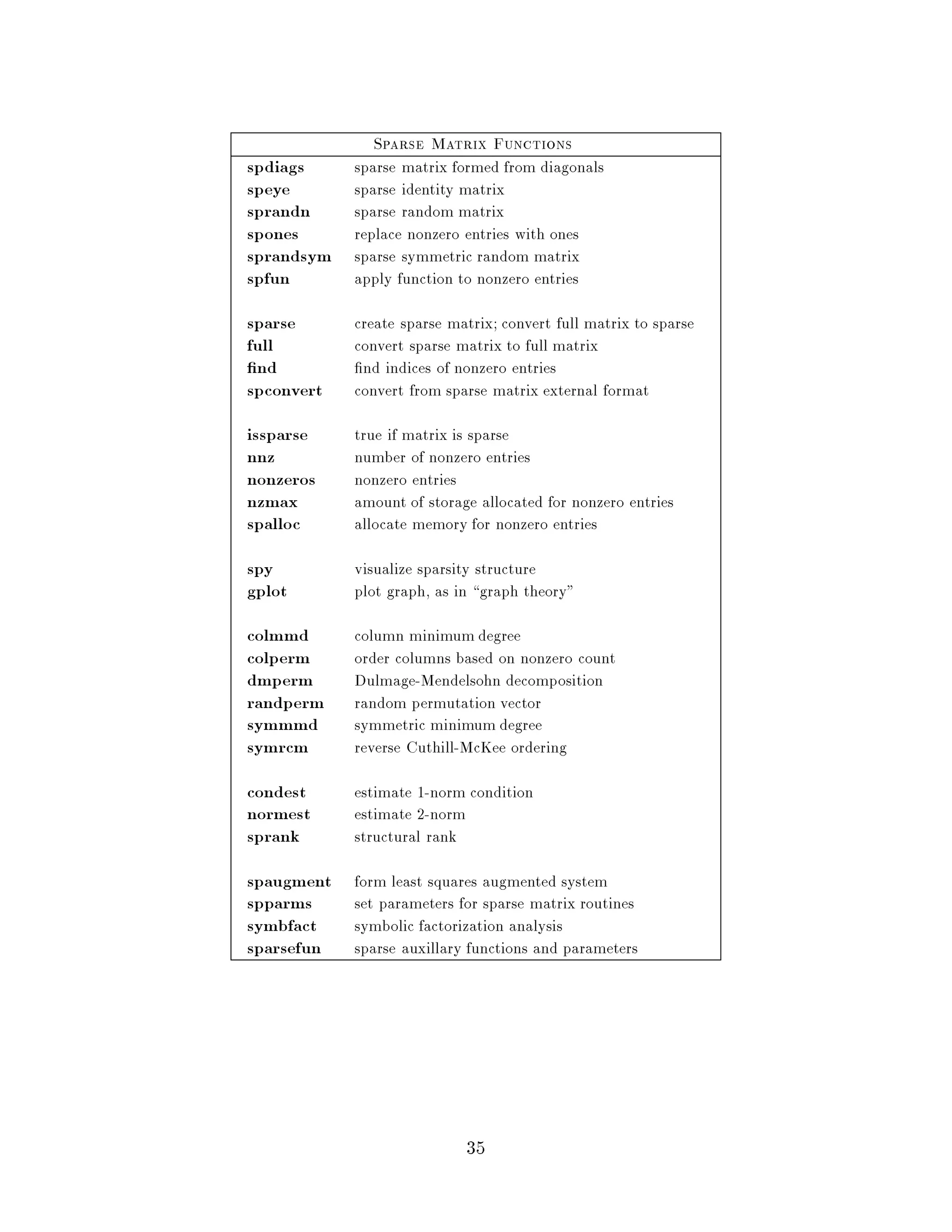
SlideShare a Scribd company logo
MATLAB Primer
               Third Edition


                          Kermit Sigmon
                     Department of Mathematics
                        University of Florida


Department of Mathematics University of Florida Gainesville, FL 32611
                        sigmon@math.ufl.edu
            Copyright c 1989, 1992, 1993 by Kermit Sigmon
On the Third Edition

    The Third Edition of the MATLAB Primer is based on version 4.0 4.1 of MATLAB.
While this edition re ects an extensive general revision of the Second Edition, most sig-
ni cant is the new information to help one begin to use the major new features of version
4.0 4.1, the sparse matrix and enhanced graphics capabilities.
    The plain TEX source and corresponding PostScript le of the latest printing of the
MATLAB Primer are always available via anonymous ftp from:
Address: math.ufl.edu Directory: pub matlab              Files: primer.tex, primer.ps
You are advised to download anew each term the latest printing of the Primer since minor
improvements and corrections may have been made in the interim. If ftp is unavailable
to you, the Primer can be obtained via listserv by sending an email message to list-
serv@math.ufl.edu containing the single line send matlab primer.tex.
    Also available at this ftp site are both English primer35.tex, primer35.ps and
Spanish primer35sp.tex, primer35sp.ps versions of the Second Edition of the Primer,
which was based on version 3.5 of MATLAB. The Spanish translation is by Celestino
Montes, University of Seville, Spain. A Spanish translation of the Third Edition is under
development.
    Users of the Primer usually appreciate the convenience and durability of a bound copy
with a cover, copy center style.
12-93


Copyright c 1989, 1992, 1993 by Kermit Sigmon
   The MATLAB Primer may be distributed as desired subject to the following con-
   ditions:
    1. It may not be altered in any way, except possibly adding an addendum giving
       information about the local computer installation or MATLAB toolboxes.
    2. It, or any part thereof, may not be used as part of a document distributed for
       a commercial purpose.
   In particular, it may be distributed via a local copy center or bookstore.

      Department of Mathematics University of Florida Gainesville, FL 32611
                              sigmon@math.ufl.edu

                                            i
Introduction
    MATLAB is an interactive, matrix-based system for scienti c and engineering numeric
computation and visualization. You can solve complex numerical problems in a fraction of
the time required with a programming language such as Fortran or C. The name MATLAB
is derived from MATrix LABoratory.
    The purpose of this Primer is to help you begin to use MATLAB. It is not intended
to be a substitute for the User's Guide and Reference Guide for MATLAB. The Primer
can best be used hands-on. You are encouraged to work at the computer as you read the
Primer and freely experiment with examples. This Primer, along with the on-line help
facility, usually su ce for students in a class requiring use of MATLAB.
    You should liberally use the on-line help facility for more detailed information. When
using MATLAB, the command help functionname will give information about a speci c
function. For example, the command help eig will give information about the eigenvalue
function eig. By itself, the command help will display a list of topics for which on-line
help is available; then help topic will list those speci c functions under this topic for which
help is available. The list of functions in the last section of this Primer also gives most of
this information. You can preview some of the features of MATLAB by rst entering the
command demo and then selecting from the options o ered.
    The scope and power of MATLAB go far beyond these notes. Eventually you will
want to consult the MATLAB User's Guide and Reference Guide. Copies of the complete
documentation are often available for review at locations such as consulting desks, terminal
rooms, computing labs, and the reserve desk of the library. Consult your instructor or your
local computing center to learn where this documentation is located at your institution.
   MATLAB is available for a number of environments: Sun Apollo VAXstation HP
workstations, VAX, MicroVAX, Gould, PC and AT compatibles, 80386 and 80486 com-
puters, Apple Macintosh, and several parallel machines. There is a relatively inexpensive
Student Edition available from Prentice Hall publishers. The information in these notes
applies generally to all of these environments.
   MATLAB is licensed by The MathWorks, Inc., 24 Prime Park Way, Natick, MA 01760,
508653-1415, Fax: 508653-2997, Email: info@mathworks.com.


   Copyright c 1989, 1992, 1993 by Kermit Sigmon
                                               ii
Contents
                                                                                                                                          Page
  1. Accessing MATLAB : : : : : : : : : : : : : : : : : : : : : : : : : : : : : : : : : : : : : : : : : : : : : : : : : : : : : : : : : : : : : 1
  2. Entering matrices : : : : : : : : : : : : : : : : : : : : : : : : : : : : : : : : : : : : : : : : : : : : : : : : : : : : : : : : : : : : : : : : 1
  3. Matrix operations, array operations : : : : : : : : : : : : : : : : : : : : : : : : : : : : : : : : : : : : : : : : : : : : : : 2
  4. Statements, expressions, variables; saving a session : : : : : : : : : : : : : : : : : : : : : : : : : : : : : : : 3
  5. Matrix building functions : : : : : : : : : : : : : : : : : : : : : : : : : : : : : : : : : : : : : : : : : : : : : : : : : : : : : : : : 4
  6. For, while, if | and relations : : : : : : : : : : : : : : : : : : : : : : : : : : : : : : : : : : : : : : : : : : : : : : : : : : : : 4
  7. Scalar functions : : : : : : : : : : : : : : : : : : : : : : : : : : : : : : : : : : : : : : : : : : : : : : : : : : : : : : : : : : : : : : : : : 7
  8. Vector functions : : : : : : : : : : : : : : : : : : : : : : : : : : : : : : : : : : : : : : : : : : : : : : : : : : : : : : : : : : : : : : : : : 7
  9. Matrix functions : : : : : : : : : : : : : : : : : : : : : : : : : : : : : : : : : : : : : : : : : : : : : : : : : : : : : : : : : : : : : : : : : 7
10. Command line editing and recall : : : : : : : : : : : : : : : : : : : : : : : : : : : : : : : : : : : : : : : : : : : : : : : : : 8
11. Submatrices and colon notation : : : : : : : : : : : : : : : : : : : : : : : : : : : : : : : : : : : : : : : : : : : : : : : : : : 8
12. M- les: script les, function les : : : : : : : : : : : : : : : : : : : : : : : : : : : : : : : : : : : : : : : : : : : : : : : : : 9
13. Text strings, error messages, input : : : : : : : : : : : : : : : : : : : : : : : : : : : : : : : : : : : : : : : : : : : : : : 12
14. Managing M- les : : : : : : : : : : : : : : : : : : : : : : : : : : : : : : : : : : : : : : : : : : : : : : : : : : : : : : : : : : : : : : : 13
15. Comparing e ciency of algorithms: ops, tic, toc : : : : : : : : : : : : : : : : : : : : : : : : : : : : : : : 14
16. Output format : : : : : : : : : : : : : : : : : : : : : : : : : : : : : : : : : : : : : : : : : : : : : : : : : : : : : : : : : : : : : : : : : 14
17. Hard copy : : : : : : : : : : : : : : : : : : : : : : : : : : : : : : : : : : : : : : : : : : : : : : : : : : : : : : : : : : : : : : : : : : : : : : 15
18. Graphics : : : : : : : : : : : : : : : : : : : : : : : : : : : : : : : : : : : : : : : : : : : : : : : : : : : : : : : : : : : : : : : : : : : : : : : 15
        planar plots 15, hardcopy 17, 3-D line plots 18
        mesh and surface plots 18, Handle Graphics 20
19. Sparse matrix computations : : : : : : : : : : : : : : : : : : : : : : : : : : : : : : : : : : : : : : : : : : : : : : : : : : : : 20
20. Reference : : : : : : : : : : : : : : : : : : : : : : : : : : : : : : : : : : : : : : : : : : : : : : : : : : : : : : : : : : : : : : : : : : : : : : 22

                                                                            iii
1. Accessing MATLAB.
    On most systems, after logging in one can enter MATLAB with the system command
matlab   and exit MATLAB with the MATLAB command quit or exit. However, your
local installation may permit MATLAB to be accessed from a menu or by clicking an icon.
    On systems permitting multiple processes, such as a Unix system or MS Windows,
you will nd it convenient, for reasons discussed in section 14, to keep both MATLAB
and your local editor active. If you are working on a platform which runs processes in
multiple windows, you will want to keep MATLAB active in one window and your local
editor active in another.
    You should consult your instructor or your local computer center for details of the local
installation.
2. Entering matrices.
    MATLAB works with essentially only one kind of object|a rectangular numerical
matrix with possibly complex entries; all variables represent matrices. In some situations,
1-by-1 matrices are interpreted as scalars and matrices with only one row or one column
are interpreted as vectors.
    Matrices can be introduced into MATLAB in several di erent ways:
        Entered by an explicit list of elements,
        Generated by built-in statements and functions,
        Created in a disk le with your local editor,
        Loaded from external data les or applications see the User's Guide.
For example, either of the statements
         A =   1 2 3; 4 5 6; 7 8 9
and
         A   =
         1   2 3
         4   5 6
         7   8 9
creates the obvious 3-by-3 matrix and assigns it to a variable A. Try it. The elements
within a row of a matrix may be separated by commas as well as a blank. When listing a
number in exponential form e.g. 2.34e-9, blank spaces must be avoided.
    MATLAB allows complex numbers in all its operations and functions. Two convenient
ways to enter complex matrices are:
         A =       1 2;3 4 + i* 5 6;7 8
         A =       1+5i 2+6i;3+7i 4+8i
When listing complex numbers e.g. 2+6i in a matrix, blank spaces must be avoided.
Either i or j may be used as the imaginary unit. If, however, you use i and j as vari-
ables and overwrite their values, you may generate a new imaginary unit with, say,
ii = sqrt-1.

                                             1
Listing entries of a large matrix is best done in an ASCII le with your local editor,
where errors can be easily corrected see sections 12 and 14. The le should consist of a
rectangular array of just the numeric matrix entries. If this le is named, say, data.ext
where .ext is any extension, the MATLAB command load data.ext will read this le
to the variable data in your MATLAB workspace. This may also be done with a script le
see section 12.
    The built-in functions rand, magic, and hilb, for example, provide an easy way to
create matrices with which to experiment. The command randn will create an n  n
matrix with randomly generated entries distributed uniformly between 0 and 1, while
randm,n will create an m  n one. magicn will create an integral n  n matrix which
is a magic square rows, columns, and diagonals have common sum; hilbn will create
the n  n Hilbert matrix, the king of ill-conditioned matrices m and n denote, of course,
positive integers. Matrices can also be generated with a for-loop see section 6 below.
    Individual matrix and vector entries can be referenced with indices inside parentheses
in the usual manner. For example, A2; 3 denotes the entry in the second row, third
column of matrix A and x3 denotes the third coordinate of vector x. Try it. A matrix
or a vector will only accept positive integers as indices.
3. Matrix operations, array operations.
   The following matrix operations are available in MATLAB:
                              +        addition
                              ,        subtraction
                                      multiplication
                              b        power
                              0        conjugate transpose
                              n        left division
                                       right division
These matrix operations apply, of course, to scalars 1-by-1 matrices as well. If the sizes
of the matrices are incompatible for the matrix operation, an error message will result,
except in the case of scalar-matrix operations for addition, subtraction, and division as
well as for multiplication in which case each entry of the matrix is operated on by the
scalar.
     The matrix division operations deserve special comment. If A is an invertible square
matrix and b is a compatible column, resp. row, vector, then
        x = Anb is the solution of A  x = b and, resp.,
        x = b=A is the solution of x  A = b.
In left division, if A is square, then it is factored using Gaussian elimination and these
factors are used to solve A  x = b. If A is not square, it is factored using Householder
orthogonalization with column pivoting and the factors are used to solve the under- or
over- determined system in the least squares sense. Right division is de ned in terms of
left division by b=A = A0 nb0 0 .

                                             2
Array operations.
    The matrix operations of addition and subtraction already operate entry-wise but the
other matrix operations given above do not|they are matrix operations. It is impor-
tant to observe that these other operations, , b , n, and , can be made to operate
entry-wise by preceding them by a period. For example, either 1,2,3,4 .* 1,2,3,4
or 1,2,3,4 .b 2 will yield 1,4,9,16 . Try it. This is particularly useful when using
Matlab graphics.
4. Statements, expressions, and variables; saving a session.
    MATLAB is an expression language; the expressions you type are interpreted and
evaluated. MATLAB statements are usually of the form
         variable = expression, or simply
         expression
Expressions are usually composed from operators, functions, and variable names. Eval-
uation of the expression produces a matrix, which is then displayed on the screen and
assigned to the variable for future use. If the variable name and = sign are omitted, a
variable ans for answer is automatically created to which the result is assigned.
    A statement is normally terminated with the carriage return. However, a statement can
be continued to the next line with three or more periods followed by a carriage return. On
the other hand, several statements can be placed on a single line if separated by commas
or semicolons.
    If the last character of a statement is a semicolon, the printing is suppressed, but the
assignment is carried out. This is essential in suppressing unwanted printing of intermediate
results.
    MATLAB is case-sensitive in the names of commands, functions, and variables. For
example, solveUT is not the same as solveut.
    The command who or whos will list the variables currently in the workspace. A
variable can be cleared from the workspace with the command clear variablename. The
command clear alone will clear all nonpermanent variables.
    The permanent variable eps epsilon gives the machine unit roundo |about 10,16 on
most machines. It is useful in specifying tolerences for convergence of iterative processes.
    A runaway display or computation can be stopped on most machines without leaving
MATLAB with CTRL-C CTRL-BREAK on a PC.
Saving a session.
    When one logs out or exits MATLAB all variables are lost. However, invoking the
command save before exiting causes all variables to be written to a non-human-readable
disk le named matlab.mat. When one later reenters MATLAB, the command load will
restore the workspace to its former state.


                                             3
5. Matrix building functions.
     Convenient matrix building functions are
                     eye           identity matrix
                     zeros         matrix of zeros
                     ones          matrix of ones
                     diag          create or extract diagonals
                     triu          upper triangular part of a matrix
                     tril          lower triangular part of a matrix
                     rand          randomly generated matrix
                     hilb          Hilbert matrix
                     magic         magic square
                     toeplitz      see help toeplitz
For example, zerosm,n produces an m-by-n matrix of zeros and zerosn produces an
n-by-n one. If A is a matrix, then zerossizeA produces a matrix of zeros having the
same size as A.
   If x is a vector, diagx is the diagonal matrix with x down the diagonal; if A is a square
matrix, then diagA is a vector consisting of the diagonal of A. What is diagdiagA?
Try it.
   Matrices can be built from blocks. For example, if A is a 3-by-3 matrix, then
        B =   A, zeros3,2; zeros2,3, eye2
will build a certain 5-by-5 matrix. Try it.
6. For, while, if | and relations.
   In their basic forms, these MATLAB ow control statements operate like those in most
computer languages.
For.
     For example, for a given n, the statement
        x =   ; for i = 1:n, x= x,ib 2 ,          end
or
        x =    ;
        for i = 1:n
            x = x,ib   2
        end
will produce a certain n-vector and the statement
        x =   ; for i = n:-1:1, x= x,ib 2 , end
will produce the same vector in reverse order. Try them. Note that a matrix may be
empty such as x = .


                                              4
The statements
         for i = 1:m
             for j = 1:n
                Hi, j = 1 i+j-1;
             end
         end
         H
will produce and print to the screen the m-by-n hilbert matrix. The semicolon on the
inner statement is essential to suppress printing of unwanted intermediate results while
the last H displays the nal result.
    The for statement permits any matrix to be used instead of 1:n. The variable just
consecutively assumes the value of each column of the matrix. For example,
         s = 0;
         for c = A
             s = s + sumc;
         end
computes the sum of all entries of the matrix A by adding its column sums Of course,
sumsumA does it more e ciently; see section 8. In fact, since 1:n = 1,2,3,: : : ,n ,
this column-by-column assigment is what occurs with if i = 1:n,: : :  see section 11.
While.
      The general form of a while loop is
         while relation
            statements
         end
The statements will be repeatedly executed as long as the relation remains true. For exam-
ple, for a given number a, the following will compute and display the smallest nonnegative
integer n such that 2n  a:
         n = 0;
         while 2b n   a
             n = n + 1;
         end
         n

If.
      The general form of a simple if statement is
         if relation
             statements
         end
The statements will be executed only if the relation is true. Multiple branching is also
possible, as is illustrated by
         if n   0
            parity = 0;

                                             5
elseif remn,2 == 0
           parity = 2;
       else
           parity = 1;
       end
In two-way branching the elseif portion would, of course, be omitted.
Relations.
   The relational operators in MATLAB are
                                   less than
                                   greater than
                              =    less than or equal
                              =    greater than or equal
                            ==     equal
                            =     not equal.
Note that = is used in an assignment statement while == is used in a relation.
Relations may be connected or quanti ed by the logical operators
                                          and
                                    j      or
                                          not.
    When applied to scalars, a relation is actually the scalar 1 or 0 depending on whether
the relation is true or false. Try entering 3 5, 3 5, 3 == 5, and 3 == 3. When
applied to matrices of the same size, a relation is a matrix of 0's and 1's giving the value
of the relation between corresponding entries. Try a = rand5, b = triua, a == b.
    A relation between matrices is interpreted by while and if to be true if each entry of
the relation matrix is nonzero. Hence, if you wish to execute statement when matrices A
and B are equal you could type
       if A == B
             statement
       end
but if you wish to execute statement when A and B are not equal, you would type
       if anyanyA      =   B
             statement
       end
or, more simply,
       if A == B else
             statement
       end
Note that the seemingly obvious
       if A = B, statement, end

                                             6
will not give what is intended since statement would execute only if each of the correspond-
ing entries of A and B di er. The functions any and all can be creatively used to reduce
matrix relations to vectors or scalars. Two any's are required above since any is a vector
operator see section 8.
7. Scalar functions.
   Certain MATLAB functions operate essentially on scalars, but operate element-wise
when applied to a matrix. The most common such functions are
     sin              asin            exp               abs             round
     cos              acos            log natural log sqrt              oor
     tan              atan            rem remainder sign              ceil

8. Vector functions.
   Other MATLAB functions operate essentially on a vector row or column, but act
on an m-by-n matrix m  2 in a column-by-column fashion to produce a row vector
containing the results of their application to each column. Row-by-row action can be
obtained by using the transpose; for example, meanA''. A few of these functions are
         max                   sum                   median               any
         min                   prod                  mean                 all
         sort                                        std
For example, the maximum entry in a matrix A is given by maxmaxA rather than
maxA. Try it.

9. Matrix functions.
   Much of MATLAB's power comes from its matrix functions. The most useful ones are
                eig        eigenvalues and eigenvectors
                chol       cholesky factorization
                svd        singular value decomposition
                inv        inverse
                lu         LU factorization
                qr         QR factorization
                hess       hessenberg form
                schur      schur decomposition
                rref       reduced row echelon form
                expm       matrix exponential
                sqrtm      matrix square root
                poly       characteristic polynomial
                det        determinant
                size       size
                norm       1-norm, 2-norm, F-norm, 1-norm
                cond       condition number in the 2-norm
                rank       rank
                                             7
MATLAB functions may have single or multiple output arguments. For example,
      y = eigA, or simply eigA
produces a column vector containing the eigenvalues of A while
         U,D     = eigA
produces a matrix U whose columns are the eigenvectors of A and a diagonal matrix D
with the eigenvalues of A on its diagonal. Try it.
10. Command line editing and recall.
    The command line in MATLAB can be easily edited. The cursor can be positioned
with the left right arrows and the Backspace or Delete key used to delete the character
to the left of the cursor. Other editing features are also available. On a PC try the Home,
End, and Delete keys; on a Unix system or a PC the Emacs commands Ctl-a, Ctl-e, Ctl-d,
and Ctl-k work; on other systems see help cedit or type cedit.
    A convenient feature is use of the up down arrows to scroll through the stack of previous
commands. One can, therefore, recall a previous command line, edit it, and execute the
revised command line. For small routines, this is much more convenient that using an
M- le which requires moving between MATLAB and the editor see sections 12 and 14.
For example, opcounts see section 15 for computing the inverse of matrices of various
sizes could be compared by repeatedly recalling, editing, and executing
        a = rand8; flops0, inva; flops
If one wanted to compare plots of the functions y = sin mx and y = sin nx on the interval
 0; 2 for various m and n, one might do the same for the command line:
        m=2; n=3; x=0:.01:2*pi; y=sinm*x; z=cosn*x; plotx,y,x,z


11. Submatrices and colon notation.
    Vectors and submatrices are often used in MATLAB to achieve fairly complex data
manipulation e ects. Colon notation which is used both to generate vectors and refer-
ence submatrices and subscripting by integral vectors are keys to e cient manipulation
of these objects. Creative use of these features to vectorize operations permits one to
minimize the use of loops which slows MATLAB and to make code simple and readable.
Special e ort should be made to become familiar with them.
    The expression 1:5 met earlier in for statements is actually the row vector 1 2 3
4 5 . The numbers need not be integers nor the increment one. For example,
        0.2:0.2:1.2
gives   0.2, 0.4, 0.6, 0.8, 1.0, 1.2       , and
        5:-1:1 gives 5 4 3 2 1 .
The following statements will, for example, generate a table of sines. Try it.
        x = 0.0:0.1:2.0 0 ;
        y = sinx;
         x y

                                             8
Note that since sin operates entry-wise, it produces a vector y from the vector x.
   The colon notation can be used to access submatrices of a matrix. For example,
       A1:4,3 is the column vector consisting of the rst four entries of the third column
       of A.
A colon by itself denotes an entire row or column:
       A:,3 is the third column of A, and A1:4,: is the rst four rows.
Arbitrary integral vectors can be used as subscripts:
       A:, 2 4  contains as columns, columns 2 and 4 of A.
Such subscripting can be used on both sides of an assignment statement:
       A:, 2 4 5  = B:,1:3 replaces columns 2,4,5 of A with the rst three columns
       of B. Note that the entire altered matrix A is printed and assigned. Try it.
Columns 2 and 4 of A can be multiplied on the right by the 2-by-2 matrix 1 2;3 4 :
       A:, 2,4  = A:, 2,4 * 1 2;3 4
Once again, the entire altered matrix is printed and assigned.
    If x is an n-vector, what is the e ect of the statement x = xn:-1:1? Try it. Also
try y = fliplrx and y = flipudx'.
    To appreciate the usefulness of these features, compare these MATLAB statements
with a Pascal, FORTRAN, or C routine to e ect the same.
12. M- les.
   MATLAB can execute a sequence of statements stored in disk les. Such les are called
 M- les because they must have the le type of .m as the last part of their lename.
Much of your work with MATLAB will be in creating and re ning M- les. M- les are
usually created using your local editor.
   There are two types of M- les: script les and function les.
Script les.
     A script le consists of a sequence of normal MATLAB statements. If the le has the
  lename, say, rotate.m, then the MATLAB command rotate will cause the statements
in the le to be executed. Variables in a script le are global and will change the value of
variables of the same name in the environment of the current MATLAB session.
     Script les may be used to enter data into a large matrix; in such a le, entry errors
can be easily corrected. If, for example, one enters in a disk le data.m
       A =
       1 2 3 4
       5 6 7 8
        ;
then the MATLAB statement data will cause the assignment given in data.m to be carried
out. However, it is usually easier to use the MATLAB function load see section 2.
    An M- le can reference other M- les, including referencing itself recursively.
                                            9
Function les.
    Function les provide extensibility to MATLAB. You can create new functions speci c
to your problem which will then have the same status as other MATLAB functions. Vari-
ables in a function le are by default local. A variable can, however, be declared global
see help global.
    We rst illustrate with a simple example of a function le.
       function a = randintm,n
       RANDINT Randomly generated integral matrix.
           randintm,n returns an m-by-n such matrix with entries
           between 0 and 9.
       a = floor10*randm,n;

   A more general version of this function is the following:
       function a = randintm,n,a,b
       RANDINT Randomly generated integral matrix.
           randintm,n returns an m-by-n such matrix with entries
           between 0 and 9.
           randm,n,a,b return entries between integers   and .     a      b
       if nargin   3, a = 0; b = 9; end
       a = floorb-a+1*randm,n + a;
This should be placed in a disk le with lename randint.m corresponding to the function
name. The rst line declares the function name, input arguments, and output arguments;
without this line the le would be a script le. Then a MATLAB statement
z = randint4,5, for example, will cause the numbers 4 and 5 to be passed to the
variables m and n in the function le with the output result being passed out to the
variable z. Since variables in a function le are local, their names are independent of those
in the current MATLAB environment.
    Note that use of nargin  number of input arguments permits one to set a default
value of an omitted input variable|such as a and b in the example.
    A function may also have multiple output arguments. For example:
       function mean, stdev = statx
        STAT Mean and standard deviation
            For a vector x, statx returns the mean of x;
             mean, stdev = statx both the mean and standard deviation.
            For a matrix x, statx acts columnwise.
         m n = sizex;
       if m == 1
           m = n;  handle case of a row vector
       end
       mean = sumx m;
                                2
       stdev = sqrtsumx.b  m - mean.b ;   2
Once this is placed in a disk le stat.m, a MATLAB command xm, xd = statx, for
example, will assign the mean and standard deviation of the entries in the vector x to
                                            10
xm and xd, respectively. Single assignments can also be made with a function having
multiple output arguments. For example, xm = statx no brackets needed around xm
will assign the mean of x to xm.
    The  symbol indicates that the rest of the line is a comment; MATLAB will ignore
the rest of the line. Moreover, the rst few contiguous comment lines, which document
the M- le, are available to the on-line help facility and will be displayed if, for example,
help stat is entered. Such documentation should always be included in a function le.
    This function illustrates some of the MATLAB features that can be used to produce
e cient code. Note, for example, that x.b 2 is the matrix of squares of the entries of x,
that sum is a vector function section 8, that sqrt is a scalar function section 7, and that
the division in sumx m is a matrix-scalar operation. Thus all operations are vectorized
and loops avoided.
    If you can't vectorize some computations, you can make your for loops go faster by
preallocating any vectors or matrices in which output is stored. For example, by including
the second statement below, which uses the function zeros, space for storing E in memory
is preallocated. Without this MATLAB must resize E one column larger in each iteration,
slowing execution.
       M = magic6;
       E = zeros6,50;
       for j = 1:50
           E:,j = eigMb i;
       end

    Some more advanced features are illustrated by the following function. As noted earlier,
some of the input arguments of a function|such as tol in this example, may be made
optional through use of nargin  number of input arguments. The variable nargout
can be similarly used. Note that the fact that a relation is a number 1 when true; 0 when
false is used and that, when while or if evaluates a relation, nonzero means true
and 0 means false. Finally, the MATLAB function feval permits one to have as an
input variable a string naming another function. Also see eval.
       function b, steps = bisectfun, x, tol
       BISECT Zero of a function of one variable via the bisection method.
           bisectfun,x returns a zero of the function. fun is a string
           containing the name of a real-valued MATLAB function of a
           single real variable; ordinarily functions are defined in
           M-files. x is a starting guess. The value returned is near
           a point where fun changes sign. For example,
           bisect'sin',3 is pi. Note the quotes around sin.
       
           An optional third input argument sets a tolerence for the
           relative accuracy of the result. The default is eps.
           An optional second output argument gives a matrix containing a
           trace of the steps; the rows are of form c fc .


                                              11
Initialization
       if nargin    3, tol = eps; end
       trace = nargout == 2;
       if x  = 0, dx = x 20; else, dx = 1 20; end
       a = x - dx; fa = fevalfun,a;
       b = x + dx; fb = fevalfun,b;

        Find change of sign.
       while fa    0 == fb   0
           dx = 2.0*dx;
           a = x - dx; fa = fevalfun,a;
           if fa   0   
                        = fb    0, break, end
           b = x + dx; fb = fevalfun,b;
       end
       if trace, steps = a fa; b fb ; end

        Main loop
       while absb - a    2.0*tol*maxabsb,1.0
           c = a + 0.5*b - a; fc = fevalfun,c;
           if trace, steps = steps; c fc ; end
           if fb   0 == fc   0
              b = c; fb = fc;
           else
              a = c; fa = fc;
           end
       end

    Some of MATLAB's functions are built-in while others are distributed as M- les. The
actual listing of any non-built-in M- le|MATLAB's or your own|can be viewed with
the MATLAB command type functionname. Try entering type eig, type vander, and
type rank.

13. Text strings, error messages, input.
   Text strings are entered into MATLAB surrounded by single quotes. For example,
       s = 'This is a test'
assigns the given text string to the variable s.
    Text strings can be displayed with the function disp. For example:
       disp'this message is hereby displayed'
Error messages are best displayed with the function error
       error'Sorry, the matrix must be symmetric'
since when placed in an M-File, it aborts execution of the M- le.


                                           12
In an M- le the user can be prompted to interactively enter input data with the function
input. When, for example, the statement
        iter = input'Enter the number of iterations:           '
is encountered, the prompt message is displayed and execution pauses while the user keys
in the input data. Upon pressing the return key, the data is assigned to the variable iter
and execution resumes.
14. Managing M- les.
    While using MATLAB one frequently wishes to create or edit an M- le with the local
editor and then return to MATLAB. One wishes to keep MATLAB active while editing a
 le since otherwise all variables would be lost upon exiting.
    This can be easily done using the !-feature. If, while in MATLAB, you precede it with
an !, any system command|such as those for editing, printing, or copying a le|can be
executed without exiting MATLAB. If, for example, the system command ed accesses your
editor, the MATLAB command
           !ed rotate.m
will let you edit the le named rotate.m using your local editor. Upon leaving the editor,
you will be returned to MATLAB just where you left it.
    However, as noted in section 1, on systems permitting multiple processes, such as one
running Unix or MS Windows, it may be preferable to keep both MATLAB and your local
editor active, keeping one process suspended while working in the other. If these processes
can be run in multiple windows, you will want to keep MATLAB active in one window
and your editor active in another.
    You should consult your instructor or your local computing center for details of the
local installation.
    Many debugging tools are available. See help dbtype or the list of functions in the
last section.
    When in MATLAB, the command pwd will return the name of the present working
directory and cd can be used to change the working directory. Either dir or ls will list
the contents of the working directory while the command what lists only the M- les in the
directory. The MATLAB commands delete and type can be used to delete a disk le and
print an M- le to the screen, respectively. While these commands may duplicate system
commands, they avoid the use of an !. You may enjoy entering the command why a few
times.
    M- les must be in a directory accessible to MATLAB. M- les in the present work-
ing directory are always accessible. On most mainframe or workstation network installa-
tions, personal M- les which are stored in a subdirectory of one's home directory named
matlab will be accessible to MATLAB from any directory in which one is working. The
current list of directories in MATLAB's search path is obtained by the command path.
This command can also be used to add or delete directories from the search path. See
help path.


                                            13
15. Comparing e ciency of algorithms: ops, tic and toc.
    Two measures of the e ciency of an algorithm are the number of oating point oper-
ations  ops performed and the elapsed time.
    The MATLAB function flops keeps a running total of the ops performed. The
command flops0 not flops = 0! will reset ops to 0. Hence, entering flops0
immediately before executing an algorithm and flops immediately after gives the op
count for the algorithm. For example, the number of ops required to solve a given linear
system via Gaussian elimination can be obtained with:
                         n
       flops0, x = A b; flops

    The elapsed time in seconds can be obtained with the stopwatch timers tic and toc;
tic starts the timer and toc returns the elapsed time. Hence, the commands
        tic, any statement, toc
will return the elapsed time for execution of the statement. The elapsed time for solving
the linear system above can be obtained, for example, with:
                   n
       tic, x = A b; toc
You may wish to compare this time|and op count|with that for solving the system
using x = invA*b;. Try it.
    It should be noted that, on timesharing machines, elapsed time may not be a reliable
measure of the e ciency of an algorithm since the rate of execution depends on how busy
the computer is at the time.
16. Output format.
    While all computations in MATLAB are performed in double precision, the format of
the displayed output can be controlled by the following commands.
        format   short           xed point with 4 decimal places the default
        format   long            xed point with 14 decimal places
        format   short e        scienti c notation with 4 decimal places
        format   long e         scienti c notation with 15 decimal places
        format   rat            approximation by ratio of small integers
        format   hex            hexadecimal format
        format   bank            xed dollars and cents
        format   +              +, -, blank
Once invoked, the chosen format remains in e ect until changed.
   The command format compact will suppress most blank lines allowing more infor-
mation to be placed on the screen or page. The command format loose returns to the
non-compact format. These commands are independent of the other format commands.


                                           14
17. Hardcopy.
    Hardcopy is most easily obtained with the diary command. The command
       diary lename
causes what appears subsequently on the screen except graphics to be written to the
named disk le if the lename is omitted it will be written to a default le named diary
until one gives the command diary off; the command diary on will cause writing to
the le to resume, etc. When nished, you can edit the le as desired and print it out on
the local system. The !-feature see section 14 will permit you to edit and print the le
without leaving MATLAB.
18. Graphics.
    MATLAB can produce planar plots of curves, 3-D plots of curves, 3-D mesh surface
plots, and 3-D faceted surface plots. The primary commands for these facilities are plot,
plot3, mesh, and surf, respectively. An introduction to each of these is given below.
    To preview some of these capabilities, enter the command demo and select some of the
graphics options.
Planar plots.
    The plot command creates linear x-y plots; if x and y are vectors of the same length,
the command plotx,y opens a graphics window and draws an x-y plot of the elements
of x versus the elements of y. You can, for example, draw the graph of the sine function
over the interval -4 to 4 with the following commands:
       x = -4:.01:4; y = sinx; plotx,y
Try it. The vector x is a partition of the domain with meshsize 0.01 while y is a vector
giving the values of sine at the nodes of this partition recall that sin operates entrywise.
    You will usually want to keep the current graphics window  gure exposed|but
moved to the side|and the command window active.
    One can have several graphics gures, one of which will at any time be the designated
 current gure where graphs from subsequent plotting commands will be placed. If, for
example, gure 1 is the current gure, then the command figure2 or simply figure
will open a second gure if necessary and make it the current gure. The command
figure1 will then expose gure 1 and make it again the current gure. The command
gcf will return the number of the current gure.
    As a second example, you can draw the graph of y = e,x2 over the interval -1.5 to 1.5
as follows:
       x = -1.5:.01:1.5; y = exp-x.b 2; plotx,y
Note that one must precede b by a period to ensure that it operates entrywise see section
3.
    MATLAB supplies a function fplot to easily and e ciently plot the graph of a function.
For example, to plot the graph of the function above, one can rst de ne the function in
an M- le called, say, expnormal.m containing
                                             15
function y = expnormalx
       y = exp-x.b 2;
Then the command
       fplot'expnormal',     -1.5,1.5 
will produce the graph. Try it.
    Plots of parametrically de ned curves can also be made. Try, for example,
       t=0:.001:2*pi; x=cos3*t; y=sin2*t; plotx,y

    The graphs can be given titles, axes labeled, and text placed within the graph with
the following commands which take a string as an argument.
        title      graph title
        xlabel     x-axis label
        ylabel     y-axis label
        gtext      place text on the graph using the mouse
        text       position text at speci ed coordinates
For example, the command
       title'Best Least Squares Fit'
gives a graph a title. The command gtext'The Spot' allows one to interactively place
the designated text on the current graph by placing the mouse pointer at the desired
position and clicking the mouse. To place text in a graph at designated coordinates, one
would use the command text see help text.
    The command grid will place grid lines on the current graph.
    By default, the axes are auto-scaled. This can be overridden by the command axis.
Some features of axis are:
        axis xmin ,xmax ,ymin ,ymax       set axis scaling to prescribed limits
        axisaxis                          freezes scaling for subsequent graphs
        axis auto                           returns to auto-scaling
        v = axis                            returns vector v showing current scaling
        axis square                        same scale on both axes
        axis equal                         same scale and tic marks on both axes
        axis off                           turns o axis scaling and tic marks
        axis on                            turns on axis scaling and tic marks
The axis command should be given after the plot command.
    Two ways to make multiple plots on a single graph are illustrated by
       x=0:.01:2*pi;y1=sinx;y2=sin2*x;y3=sin4*x;plotx,y1,x,y2,x,y3
and by forming a matrix Y containing the functional values as columns
       x=0:.01:2*pi; Y= sinx', sin2*x', sin4*x' ; plotx,Y
Another way is with hold. The command hold on freezes the current graphics screen so
that subsequent plots are superimposed on it. The axes may, however, become rescaled.
Entering hold off releases the hold.

                                           16
One can override the default linetypes, pointtypes and colors. For example,
       x=0:.01:2*pi; y1=sinx; y2=sin2*x; y3=sin4*x;
       plotx,y1,'--',x,y2,':',x,y3,'+'
renders a dashed line and dotted line for the rst two graphs while for the third the symbol
+ is placed at each node. The line- and mark-types are
        Linetypes: solid -, dashed --. dotted :, dashdot -.
        Marktypes: point ., plus +, star *, circle o, x-mark x
Colors can be speci ed for the line- and mark-types.
        Colors: yellow y, magenta m, cyan c, red r
                 green g, blue b, white w, black k
For example, plotx,y,'r--' plots a red dashed line.
    The command subplot can be used to partition the screen so that several small plots
can be placed in one gure. See help subplot.
    Other specialized 2-D plotting functions you may wish to explore via help are:
       polar, bar, hist, quiver, compass, feather, rose, stairs, fill

Graphics hardcopy
     A hardcopy of the current graphics gure can be most easily obtained with the MAT-
LAB command print. Entered by itself, it will send a high-resolution copy of the current
graphics gure to the default printer.
     The printopt M- le is used to specify the default setting used by the print command.
If desired, one can change the defaults by editing this le see help printopt.
     The command print lename saves the current graphics gure to the designated
  lename in the default le format. If lename has no extension, then an appropriate
extension such as .ps, .eps, or .jet is appended. If, for example, PostScript is the
default le format, then
       print lissajous
will create a PostScript le lissajous.ps of the current graphics gure which can subse-
quently be printed using the system print command. If filename already exists, it will be
overwritten unless you use the -append option. The command
       print -append lissajous
will append the hopefully di erent current graphics gure to the existing le
lissajous.ps. In this way one can save several graphics gures in a single le.
    The default settings can, of course, be overwritten. For example,
       print -deps -f3 saddle
will save to an Encapsulated PostScript le saddle.eps the graphics gure 3 | even if it
is not the current gure.


                                            17
3-D line plots.
    Completely analogous to plot in two dimensions, the command plot3 produces curves
in three dimensional space. If x, y, and z are three vectors of the same size, then the
command plot3x,y,z will produce a perspective plot of the piecewise linear curve in
3-space passing through the points whose coordinates are the respective elements of x, y,
and z. These vectors are usually de ned parametrically. For example,
       t=.01:.01:20*pi; x=cost; y=sint; z=t.b 3; plot3x,y,z
will produce a helix which is compressed near the x-y plane a slinky. Try it.
    Just as for planar plots, a title and axis labels including zlabel can be added. The
features of axis command described there also hold for 3-D plots; setting the axis scaling
to prescribed limits will, of course, now require a 6-vector.
3-D mesh and surface plots.
    Three dimensional wire mesh surface plots are drawn with the command mesh. The
command meshz creates a three-dimensional perspective plot of the elements of the
matrix z. The mesh surface is de ned by the z-coordinates of points above a rectangular
grid in the x-y plane. Try mesheye10.
    Similarly, three dimensional faceted surface plots are drawn with the command surf.
Try surfeye10.
    To draw the graph of a function z = f x; y over a rectangle, one rst de nes vectors
xx and yy which give partitions of the sides of the rectangle. With the function meshgrid
one then creates a matrix x, each row of which equals xx and whose column length is the
length of yy, and similarly a matrix y, each column of which equals yy, as follows:
        x,y   = meshgridxx,yy;
One then computes a matrix z, obtained by evaluating f entrywise over the matrices x
and y, to which mesh or surf can be applied.
    You can, for example, draw the graph of z = e,x2 ,y2 over the square ,2; 2  ,2; 2
as follows try it:
       xx = -2:.2:2;
       yy = xx;
        x,y = meshgridxx,yy;
       z = exp-x.b 2 - y.b 2;
       meshz
One could, of course, replace the rst three lines of the preceding with
        x,y   = meshgrid-2:.2:2, -2:.2:2;
Try this plot with surf instead of mesh.
    As noted above, the features of the axis command described in the section on planar
plots also hold for 3-D plots as do the commands for titles, axes labelling and the command
hold.
    The color shading of surfaces is set by the shading command. There are three settings
for shading: faceted default, interpolated, and flat. These are set by the commands
                                            18
shading faceted,     shading interp,        or shading flat
Note that on surfaces produced by surf, the settings interpolated and flat remove
the superimposed mesh lines. Experiment with various shadings on the surface produced
above. The command shading as well as colormap and view below should be entered
after the surf command.
    The color pro le of a surface is controlled by the colormap command. Available pre-
de ned colormaps include:
        hsv default, hot, cool, jet, pink, copper, flag, gray, bone
The command colormapcool will, for example, set a certain color pro le for the current
 gure. Experiment with various colormaps on the surface produced above.
    The command view can be used to specify in spherical or cartesian coordinates the
viewpoint from which the 3-D object is to be viewed. See help view.
    The MATLAB function peaks generates an interesting surface on which to experiment
with shading, colormap, and view.
    Plots of parametrically de ned surfaces can also be made. The MATLAB functions
sphere and cylinder will generate such plots of the named surfaces. See type sphere
and type cylinder. The following is an example of a similar function which generates a
plot of a torus.
       function x,y,z = torusr,n,a
       TORUS Generate a torus
          torusr,n,a generates a plot of a torus with central
          radius a and lateral radius r. n controls the number
          of facets on the surface. These input variables are optional
          with defaults r = 0.5, n = 30, a = 1.
       
           x,y,z = torusr,n,a generates three n+1-by-n+1
          matrices so that surfx,y,z will produce the torus.
       
          See also SPHERE, CYLINDER

       if nargin   3, a = 1; end
       if nargin   2, n = 30; end
       if nargin   1, r = 0.5; end
       theta = pi*0:2:2*n n;
       phi = 2*pi*0:2:n' n;
       xx = a + r*cosphi*costheta;
       yy = a + r*cosphi*sintheta;
       zz = r*sinphi*onessizetheta;
       if nargout == 0
          surfxx,yy,zz
          ar = a + r sqrt2;
          axis -ar,ar,-ar,ar,-ar,ar 
       else

                                          19
x = xx; y = yy; z = zz;
       end

   Other 3-D plotting functions you may wish to explore via help are:
       meshz, surfc, surfl, contour, pcolor

Handle Graphics.
   Beyond those described above, MATLAB's graphics system provides low level functions
which permit one to control virtually all aspects of the graphics environment to produce
sophisticated plots. Enter the command set1 and gca,setans to see some of the
properties of gure 1 which one can control. This system is called Handle Graphics, for
which one is referred to the MATLAB User's Guide.
19. Sparse Matrix Computations.
    In performing matrix computations, MATLAB normally assumes that a matrix is
dense; that is, any entry in a matrix may be nonzero. If, however, a matrix contains
su ciently many zero entries, computation time could be reduced by avoiding arithmetic
operations on zero entries and less memory could be required by storing only the nonzero
entries of the matrix. This increase in e ciency in time and storage can make feasible
the solution of signi cantly larger problems than would otherwise be possible. MATLAB
provides the capability to take advantage of the sparsity of matrices.
    Matlab has two storage modes, full and sparse, with full the default. The functions
full and sparse convert between the two modes. For a matrix A, full or sparse, nnzA
returns the number of nonzero elements in A.
    A sparse matrix is stored as a linear array of its nonzero elements along with their row
and column indices. If a full tridiagonal matrix F is created via, say,
       F = floor10*rand6; F = triutrilF,1,-1;
then the statement S = sparseF will convert F to sparse mode. Try it. Note that the
output lists the nonzero entries in column major order along with their row and column
indices. The statement F = fullS restores S to full storage mode. One can check the
storage mode of a matrix A with the command issparseA.
    A sparse matrix is, of course, usually generated directly rather than by applying the
function sparse to a full matrix. A sparse banded matrix can be easily created via the
function spdiags by specifying diagonals. For example, a familiar sparse tridiagonal matrix
is created by
       m = 6; n = 6; e = onesn,1; d = -2*e;
       T = spdiags e,d,e , -1,0,1 ,m,n
Try it. The integral vector -1,0,1 speci es in which diagonals the columns of e,d,e should
be placed use fullT to view. Experiment with other values of m and n and, say, -3,0,2
instead of -1,0,1 . See help spdiags for further features of spdiags.


                                            20
The sparse analogs of eye, zeros, ones, and randn for full matrices are, respectively,
       speye,     sparse,    spones,     sprandn
The latter two take a matrix argument and replace only the nonzero entries with ones
and normally distributed random numbers, respectively. randn also permits the sparsity
structure to be randomized. The command sparsem,n creates a sparse zero matrix.
    The versatile function sparse permits creation of a sparse matrix via listing its nonzero
entries. Try, for example,
       i = 1 2 3 4 4 4 ; j = 1 2 3 1 2 3 ; s =                 5 6 7 8 9 10 ;
       S = sparsei,j,s,4,3, fullS
In general, if the vector s lists the nonzero entries of S and the integral vectors i and j list
their corresponding row and column indices, then
       sparsei,j,s,m,n
will create the desired sparse m  n matrix S . As another example try
       n = 6; e = floor10*randn-1,1; E = sparse2:n,1:n-1,e,n,n

     The arithmetic operations and most MATLAB functions can be applied independent
of storage mode. The storage mode of the result? Operations on full matrices always give
full results. Selected other results are S=sparse, F=full:
        Sparse: S+S, S*S, S.*S, S.*F, Sb n, S.b n, SnS
        Full: S+F, S*F, SnF, FnS
        Sparse: invS, cholS, luS, diagS, maxS, sumS
For sparse S , eigS is full if S is symmetric but unde ned if S is unsymmetric; svd
requires a full argument. A matrix built from blocks, such as A,B;C,D , is sparse if any
constituent block is sparse.
     You may wish to compare, for the two storage modes, the e ciency of solving a tridi-
agonal system of equations for, say, n = 20; 50; 500; 1000 by entering, recalling and editing
the following two command lines:
       n=20;e=onesn,1;d=-2*e; T=spdiags e,d,e , -1,0,1 ,n,n; A=fullT;
                                             n
       b=onesn,1;s=sparseb;tic,T s;sparsetime=toc, tic,A b;fulltime=tocn


                                                 21
20. Reference.
    There are many MATLAB features which cannot be included in these introductory
notes. Listed below are some of the MATLAB functions and operators available, grouped
by subject area1. Use the on-line help facility or consult the Reference Guide for more
detailed information on the functions.
    There are many functions beyond these. There exist, in particular, several toolboxes
of functions for speci c areas2. Included among such are signal processing, control systems,
robust-control, system identi cation, optimization, splines, chemometrics, -analysis and
synthesis, state-space identi cation, neural networks, image processing, symbolic math
Maple kernel, and statistics. These can be explored via the command help.

                              Managing Commands and Functions
                  help           help facility
                  what           list M- les on disk
                  type           list named M- le
                  lookfor        keywork search through the help entries
                  which          locate functions and les
                  demo           run demonstrations
                  path           control MATLAB's search path
                  cedit          set parameters for command line editing and recall
                  version        display MATLAB version you are running
                  whatsnew       display toolbox README les
                  info           info about MATLAB and The MathWorks
                  why            receive ippant answer


                            Managing Variables and the Workspace
                        who        list current variables
                        whos       list current variables, long form
                        save       save workspace variables to disk
                        load       retrieve variables from disk
                        clear      clear variables and functions from memory
                        pack       consolidate workspace memory
                        size       size of matrix
                        length     length of vector
                        disp       display matrix or text

 1 Source: MATLAB Reference Guide, version 4.1
 2 The toolboxes, which are optional, may not be installed on your system.

                                                  22
Working with Files and the Operating System
cd            change current working directory
pwd           show current working directory
dir, ls       directory listing
delete        delete le
getenv        get environment variable
!             execute operating system command
unix          execute operating system command; return result
diary         save text of MATLAB session

           Controlling the Command Window
     clc         clear command window
     home        send cursor home|to top of screen
     format      set output format
     echo        echo commands inside script commands
     more        control paged output in command window

          Starting and Quitting from MATLAB
  quit            terminate MATLAB
  startup         M- le executed when MATLAB is started
  matlabrc        master startup M- le

          Matrix Operators               Array Operators
 +         addition                      +     addition
 ,         subtraction                   ,     subtraction
          multiplication                .    multiplication
 b         power                         .b    power
           right division                .     right division
 n         left division                 .n    left division
 '         conjugate transpose
 .'        transpose
 kron      Kronecker tensor product

           Relational and Logical Operators
              less than                   and
        = less than or equal           j   or
              greater than                not
       = greater than or equal         xor exclusive or
      == equal
      = not equal
                               23
Special Characters
=     assignment statement
      used to form vectors and matrices; enclose multiple function output variables
    arithmetic expression precedence; enclose function input variables
.     decimal point
..    parent directory
...   continue statement to next line
,     separate subscripts, function arguments, statements
;     end rows, suppress printing
     comments
:     subscripting, vector generation
!     execute operating system command


                    Special Variables and Constraints
             ans             answer when expression not assigned
             eps               oating point precision
             realmax         largest oating point number
             reammin         smallest positive oating point number
             pi              
             i, j            imaginary unit
             inf             in nity
             NaN             Not-a-Number
               ops            oating point operation count
             nargin          number of function input arguments
             nargout         number of function output arguments
             computer        computer type


                                 Time and Date
                     date         current date
                     clock        wall clock
                     etime        elapsed time function
                     tic, toc     stopwatch timer functions
                     cputime      elapsed CPU time

                                        24
Special Matrices
zeros        matrix of zeros
ones         matrix of ones
eye          identity
diag         diagonal
toeplitz     Toeplitz
magic        magic square
compan       companion
linspace     linearly spaced vectors
logspace     logarithmically spaced vectors
meshgrid     array for 3-D plots
rand         uniformly distributed random numbers
randn        normally distributed randon numbers
hilb         Hilbert
invhilb      inverse Hilbert exact
vander       Vandermonde
pascal       Pascal
hadamard     Hadamard
hankel       Hankel
rosser       symmetric eigenvalue test matrix
wilkinson    Wilkinson's eigenvalue test matrix
gallery      two small test matrices


            Matrix Manipulation
 diag       create or extract diagonals
 rot90      rotate matrix 90 degrees
    iplr      ip matrix left-to-right
    ipud      ip matrix up-to-down
 reshape    change size
 tril       lower triangular part
 triu       upper triangular part
 .'         transpose
 :          convert matrix to single column; A:


                       25
Logical Functions
  exist       check if variables or functions exist
  any         true if any element of vector is true
  all         true if all elements of vector are true
    nd         nd indices of non-zero elements
  isnan       true for NaNs
  isinf       true for in nite elements
    nite      true for nite elements
  isieee      true for IEEE oating point arithmetic
  isempty     true for empty matrix
  issparse    true for sparse matrix
  isstr       true for text string
  strcmp      compare string variables


                  Control Flow
if       conditionally execute statements
else     used with if
elseif   used with if
end      terminate if, for, while
for      repeat statements for a speci c number of times
while    repeat statments while condition is true
break    terminate execution of for or while loops
return   return to invoking function
error    display message and abort function


                   Programming
 input       prompt for user input
 keyboard    invoke keyboard as if it were a script le
 menu        generate menu of choices for user input
 pause       wait for user response
 function    de ne function
 eval        execute string with MATLAB expression
 feval       evaluate function speci ed by string
 global      de ne global variables
 nargchk     validate number of input arguments

                          26
Text and Strings
string     about character strings in MATLAB
abs        convert string to numeric values
blanks     a string of blanks
eval       evaluate string with MATLAB expression
num2str    convert number to string
int2str    convert integer to string
str2num    convert string to number
isstr      true for string variables
strcmp     compare string variables
upper      convert string to uppercase
lower      convert string to lowercase
hex2num    convert hex string to oating point number
hex2dec    convert hex string to decimal integer
dec2hex    convert decimal integer to hex string


                   Debugging
    dbstop      set breakpoint
    dbclear     remove breakpoint
    dbcont      remove execution
    dbdown      change local workspace context
    dbstack     list who called whom
    dbstatus    list all breakpoints
    dbstep      execute one or more lines
    dbtype      list M- le with line numbers
    dbup        change local workspace context
    dbdown      opposite of dbup
    dbquit      quit debug mode


          Sound Processing Functions
     saxis        sound axis scaling
     sound        convert vector to sound
     auread       Read Sun audio le
     auwrite      Write Sun audio le
     lin2mu       linear to mu-law conversion
     mu2lin       mu-law to linear conversion

                        27
Elementary Math Functions
                    abs            absolute value or complex magnitude
                    angle          phase angle
                    sqrt           square root
                    real           real part
                    imag           imaginary part
                    conj           complex conjugate
                    gcd            greatest common divisor
                    lcm            least common multiple
                    round          round to nearest integer
                      x            round toward zero
                      oor          round toward ,1
                    ceil           round toward 1
                    sign           signum function
                    rem            remainder
                    exp            exponential base e
                    log            natural logarithm
                    log10          log base 10


                              Trigonometric Functions
sin, asin, sinh, asinh     sine, arcsine, hyperbolic sine, hyperbolic arcsine
cos, acos, cosh, acosh     cosine, arccosine, hyperbolic cosine, hyperbolic arccosine
tan, atan, tanh, atanh     tangent, arctangent, hyperbolic tangent, hyperbolic arctangent
cot, acot, coth, acoth     cotangent, arccotangent, hyperbolic cotan., hyperbolic arccotan.
sec, asec, sech, asech     secant, arcsecant, hyperbolic secant, hyperbolic arcsecant
csc, acsc, csch, acsch     cosecant, arccosecant, hyperbolic cosecant, hyperbolic arccosecant


                                     Special Functions
                         bessel       bessel function
                         beta         beta function
                         gamma        gamma function
                         rat          rational approximation
                         rats         rational output
                         erf          error function
                         erfinv       inverse error function
                         ellipke      complete elliptic integral
                         ellipj       Jacobian elliptic integral
                         expint       exponential integral
                         log2         dissect oating point numbers
                         pow2         scale oating point numbers

                                              28
Matrix Decompositions and Factorizations
inv        inverse
lu         factors from Gaussian elimination
rref       reduced row echelon form
chol       Cholesky factorization
qr         orthogonal-triangular decomposition
nnls       nonnegative least squares
lscov      least squares in presence of know covariance
null       null space
orth       orthogonalization
eig        eigenvalues and eigenvectors
hess       Hessenberg form
schur      Schur decomposition
cdf2rdf    complex diagonal form to real block diagonal form
rsf2csf    real block diagonal form to complex diagonal form
balance    diagonal scaling for eigenvalue accuracy
qz         generalized eigenvalues
polyeig    polynomial eigenvalue solver
svd        singular value decomposition
pinv       pseudoinverse


                  Matrix Conditioning
cond        condition number in 2-norm
rcond       LINPACK reciprocal condition number estimator
condest     Hager Higham condition number estimator
norm        1-norm,2-norm,F-norm,1-norm
normest     2-norm estimator
rank        rank


            Elementary Matrix Functions
expm      matrix exponential
expm1     M- le implementation of expm
expm2     matrix exponential via Taylor series
expm3     matrix exponential via eigenvalues and eigenvectors
logm      matrix logarithm
sqrtm     matrix square root
funm      evaluate general matrix function
poly      characteristic polynomial
det       determinant
trace     trace

                             29
Polynomials
  poly         construct polynomial with speci ed roots
  roots        polynomial roots|companion matrix method
  roots1       polynomial roots|Laguerre's method
  polyval      evaluate polynomial
  polyvalm     evaluate polynomial with matrix argument
  conv         multiply polynomials
  deconv       divide polynomials
  residue      partial-fraction expansion residues
  poly t        t polynomial to data
  polyder      di erentiate polynomial

              Column-wise Data Analysis
       max           largest component
       min           smallest component
       mean          average or mean value
       median        median value
       std           standard deviation
       sort          sort in ascending order
       sum           sum of elements
       prod          product of elements
       cumsum        cumulative sum of elements
       cumprod       cumulative product of elements
       hist          histogram

                   Signal Processing
abs          complex magnitude
angle        phase angle
conv         convolution and polynomial multiplication
deconv       deconvolution and polynomial division
corrcoef     correlation coe cients
cov          covariance matrix
 lter        one-dimensional digital lter
 lter2       two-dimensional digital lter
cplxpair     sort numbers into complex pairs
unwrap       remove phase angle jumps across 360 boundaries
nextpow2     next higher power of 2
 t           radix-2 fast Fourier transform
 t2          two-dimensional FFT
i t          inverse fast Fourier transform
i t2         inverse 2-D FFT
 tshift      zero-th lag to center of spectrum

                            30
Finite Differences and Data Interpolation
di            approximate derivatives
gradient      approximate gradient
del2           ve point discrete Laplacian
subspace      angle between two subspaces
spline        cubic spline interpolation
interp1       1-D data interpolation
interp2       2-D data interpolation
interpft      1-D data interpolation via FFT method
griddata      data gridding


              Numerical Integration
   quad       adaptive 2-panel Simpson's Rule
   quad8      adaptive 8-panel Newton-Cotes Rule
   trapz      trapezoidal method


         Differential Equation Solution
ode23 2nd 3rd order Runge-Kutta method
ode23p solve via ode23, displaying plot
ode45 4th 5th order Runge-Kutta-Fehlberg method


    Nonlinear Equations and Optimization
fmin       minimize function of one variable
fmins      minimize function of several variables
fsolve     solution to a system of nonlinear equations
            nd zeros of a function of several variables
fzero       nd zero of function of one variable
fplot      plot graph of a function


                           31
Two Dimensional Graphs
    plot         linear plot
    loglog       log-log scale plot
    semilogx     semilog scale plot
    semilogy     semilog scale plot
      ll         draw lled 2-D polygons
    polar        polar coordinate plot
    bar          bar graph
    stairs       stairstep plot
    errorbar     error bar plot
    hist         histogram plot
    rose         angle histogram plot
    compass      compass plot
    feather      feather plot
    fplot        plot function


             Graph Annotation
    title      graph title
    xlabel     x-axis label
    ylabel     y-axis label
    zlabel     z-axis label for 3-D plots
    grid       grid lines
    text       text annotation
    gtext      mouse placement of text
    ginput     graphical input from mouse


Figure Window Axis Creation and Control
  gure     create gure graph window
gcf        get handle to current gure
clf        clear current gure
close      close gure
hold       hold current graph
ishold     return hold status
subplot    create axes in tiled positions
axes       create axes in arbitrary positions
gca        get handle to to current axes
axis       control axis scaling and appearance
caxis      control pseudocolor axis scaling

                      32
Graph Hardcopy and Storage
      print    print graph or save graph to le
      printopt con gure local printer defaults
      orient   set paper orientation


             Three Dimensional Graphs
mesh        3-D mesh surface
meshc       combination mesh contour plot
meshz       3-D mesh with zero plane
surf        3-D shaded surface
surfc       combination surface contour plot
surfl       3-D shaded surface with lighting
plot3       plot lines and points in 3-D space
  ll3       draw lled 3-D polygons in 3-D space
contour     contour plot
contour3    3-D contour plot
clabel      contour plot elevation labels
contourc    contour plot computation used by contour
pcolor      pseudocolor checkerboard plot
quiver      quiver plot
image       display image
waterfall   waterfall plot
slice       volumetric visualization plot


                3-D Graph Appearance
     view         3-D graph viewpoint speci cation
     viewmtx      view transformation matrices
     hidden       mesh hidden line removal mode
     shading      color shading mode
     axis         axis scaling and apearance
     caxis        pseudocolor axis scaling
     specular     specular re ectance
     di use       di use re ectance
     surfnorm     surface normals
     colormap     color lookup table see below
     brighten     brighten or darken color map
     spinmap      spin color map
     rgbplot      plot colormap
     hsv2rgb      hsv to rgb color map conversion
     rgb2hsv      rgb to hsv color map conversion

                          33
Color Maps
hsv        hue-saturation-value default
jet        variant of hsv
gray       linear gray-scale
hot        black-red-yellow-white
cool       shades of cyan and magenta
bone       gray-scale with tinge of blue
copper     linear copper tone
pink       pastel shades of pink
  ag       alternating red, white, blue, and black


                 3-D Objects
     sphere generate sphere
     cylinder generate cylinder
     peaks    generate demo surface


            Movies and Animation
  moviein       initialize movie frame memory
  getframe      get movie frame
  movie         play recorded movie frames


          Handle Graphics Objects
     gure        create gure window
   axes          create axes
   line          create line
   text          create text
   patch         create patch
   surface       create surface
   image         create image
   uicontrol     create user interface control
   uimenu        create user interface menu


         Handle Graphics Operations
  set           set object properties
  get           get object properties
  reset         reset object properties
  delete        delete object
  drawnow        ush pending graphics events

                       34
Sparse Matrix Functions
spdiags     sparse matrix formed from diagonals
speye       sparse identity matrix
sprandn     sparse random matrix
spones      replace nonzero entries with ones
sprandsym   sparse symmetric random matrix
spfun       apply function to nonzero entries
sparse      create sparse matrix; convert full matrix to sparse
full        convert sparse matrix to full matrix
 nd          nd indices of nonzero entries
spconvert   convert from sparse matrix external format
issparse    true if matrix is sparse
nnz         number of nonzero entries
nonzeros    nonzero entries
nzmax       amount of storage allocated for nonzero entries
spalloc     allocate memory for nonzero entries

spy         visualize sparsity structure
gplot       plot graph, as in graph theory
colmmd      column minimum degree
colperm     order columns based on nonzero count
dmperm      Dulmage-Mendelsohn decomposition
randperm    random permutation vector
symmmd      symmetric minimum degree
symrcm      reverse Cuthill-McKee ordering

condest     estimate 1-norm condition
normest     estimate 2-norm
sprank      structural rank
spaugment   form least squares augmented system
spparms     set parameters for sparse matrix routines
symbfact    symbolic factorization analysis
sparsefun   sparse auxillary functions and parameters


                            35

More Related Content

Viewers also liked

Image Processing Using MATLAB
Image Processing Using MATLABImage Processing Using MATLAB
Image Processing Using MATLAB
Amarjeetsingh Thakur
 
Matlab Working With Images
Matlab Working With ImagesMatlab Working With Images
Matlab Working With Images
matlab Content
 
Digital image processing using matlab
Digital image processing using matlab Digital image processing using matlab
Digital image processing using matlab
Amr Rashed
 
Image enhancement techniques
Image enhancement techniquesImage enhancement techniques
Image enhancement techniques
Saideep
 
Basics of Image Processing using MATLAB
Basics of Image Processing using MATLABBasics of Image Processing using MATLAB
Basics of Image Processing using MATLAB
vkn13
 
Image proceesing with matlab
Image proceesing with matlabImage proceesing with matlab
Image proceesing with matlab
Ashutosh Shahi
 
Digital Image Processing Fundamental
Digital Image Processing FundamentalDigital Image Processing Fundamental
Digital Image Processing Fundamental
Thuong Nguyen Canh
 
Introduction to Digital Image Processing Using MATLAB
Introduction to Digital Image Processing Using MATLABIntroduction to Digital Image Processing Using MATLAB
Introduction to Digital Image Processing Using MATLAB
Ray Phan
 
Digital Image Processing
Digital Image ProcessingDigital Image Processing
Digital Image Processing
Sahil Biswas
 
Image processing ppt
Image processing pptImage processing ppt
Image processing ppt
Raviteja Chowdary Adusumalli
 

Viewers also liked (10)

Image Processing Using MATLAB
Image Processing Using MATLABImage Processing Using MATLAB
Image Processing Using MATLAB
 
Matlab Working With Images
Matlab Working With ImagesMatlab Working With Images
Matlab Working With Images
 
Digital image processing using matlab
Digital image processing using matlab Digital image processing using matlab
Digital image processing using matlab
 
Image enhancement techniques
Image enhancement techniquesImage enhancement techniques
Image enhancement techniques
 
Basics of Image Processing using MATLAB
Basics of Image Processing using MATLABBasics of Image Processing using MATLAB
Basics of Image Processing using MATLAB
 
Image proceesing with matlab
Image proceesing with matlabImage proceesing with matlab
Image proceesing with matlab
 
Digital Image Processing Fundamental
Digital Image Processing FundamentalDigital Image Processing Fundamental
Digital Image Processing Fundamental
 
Introduction to Digital Image Processing Using MATLAB
Introduction to Digital Image Processing Using MATLABIntroduction to Digital Image Processing Using MATLAB
Introduction to Digital Image Processing Using MATLAB
 
Digital Image Processing
Digital Image ProcessingDigital Image Processing
Digital Image Processing
 
Image processing ppt
Image processing pptImage processing ppt
Image processing ppt
 

Similar to Primer

Malab tutorial
Malab tutorialMalab tutorial
Malab tutorial
sisira senarathna
 
EE6711 Power System Simulation Lab manual
EE6711 Power System Simulation Lab manualEE6711 Power System Simulation Lab manual
EE6711 Power System Simulation Lab manual
Velalar College of Engineering and Technology
 
interfacing matlab with embedded systems
interfacing matlab with embedded systemsinterfacing matlab with embedded systems
interfacing matlab with embedded systems
Raghav Shetty
 
Matlab anilkumar
Matlab  anilkumarMatlab  anilkumar
Matlab anilkumar
THEMASTERBLASTERSVID
 
MATLAB Workshop yugjjnhhasfhlhhlllhl.pptx
MATLAB Workshop yugjjnhhasfhlhhlllhl.pptxMATLAB Workshop yugjjnhhasfhlhhlllhl.pptx
MATLAB Workshop yugjjnhhasfhlhhlllhl.pptx
prashantkumarchinama
 
Matlab tut2
Matlab tut2Matlab tut2
Matlab tut2
Vinnu Vinay
 
Fulltext
FulltextFulltext
MATLAB Assignment Help
MATLAB Assignment HelpMATLAB Assignment Help
MATLAB Assignment Help
Essay Corp
 
Kevin merchantss
Kevin merchantssKevin merchantss
Kevin merchantss
dharmesh69
 
KEVIN MERCHANT DOCUMENT
KEVIN MERCHANT DOCUMENTKEVIN MERCHANT DOCUMENT
KEVIN MERCHANT DOCUMENT
tejas1235
 
Matlab summary
Matlab summaryMatlab summary
Matlab summary
Vinnu Vinay
 
Matlab
MatlabMatlab
An Introduction to MATLAB with Worked Examples
An Introduction to MATLAB with Worked ExamplesAn Introduction to MATLAB with Worked Examples
An Introduction to MATLAB with Worked Examples
eAssessment in Practice Symposium
 
Matlab - Introduction and Basics
Matlab - Introduction and BasicsMatlab - Introduction and Basics
Matlab - Introduction and Basics
Techsparks
 
Introduction to Matlab for Engineering Students.pdf
Introduction to Matlab for Engineering Students.pdfIntroduction to Matlab for Engineering Students.pdf
Introduction to Matlab for Engineering Students.pdf
DrAzizulHasan1
 
Matlab Introduction
Matlab IntroductionMatlab Introduction
Matlab Introduction
ideas2ignite
 
Systems interfacesanddeployment
Systems interfacesanddeploymentSystems interfacesanddeployment
Systems interfacesanddeployment
Xavier Davias
 
Signals and systems with matlab computing and simulink modeling
Signals and systems with matlab computing and simulink modelingSignals and systems with matlab computing and simulink modeling
Signals and systems with matlab computing and simulink modeling
votasugs567
 
HPC and HPGPU Cluster Tutorial
HPC and HPGPU Cluster TutorialHPC and HPGPU Cluster Tutorial
HPC and HPGPU Cluster Tutorial
Dirk Hähnel
 
Introduction to MATrices LABoratory (MATLAB) as Part of Digital Signal Proces...
Introduction to MATrices LABoratory (MATLAB) as Part of Digital Signal Proces...Introduction to MATrices LABoratory (MATLAB) as Part of Digital Signal Proces...
Introduction to MATrices LABoratory (MATLAB) as Part of Digital Signal Proces...
Ahmed Gad
 

Similar to Primer (20)

Malab tutorial
Malab tutorialMalab tutorial
Malab tutorial
 
EE6711 Power System Simulation Lab manual
EE6711 Power System Simulation Lab manualEE6711 Power System Simulation Lab manual
EE6711 Power System Simulation Lab manual
 
interfacing matlab with embedded systems
interfacing matlab with embedded systemsinterfacing matlab with embedded systems
interfacing matlab with embedded systems
 
Matlab anilkumar
Matlab  anilkumarMatlab  anilkumar
Matlab anilkumar
 
MATLAB Workshop yugjjnhhasfhlhhlllhl.pptx
MATLAB Workshop yugjjnhhasfhlhhlllhl.pptxMATLAB Workshop yugjjnhhasfhlhhlllhl.pptx
MATLAB Workshop yugjjnhhasfhlhhlllhl.pptx
 
Matlab tut2
Matlab tut2Matlab tut2
Matlab tut2
 
Fulltext
FulltextFulltext
Fulltext
 
MATLAB Assignment Help
MATLAB Assignment HelpMATLAB Assignment Help
MATLAB Assignment Help
 
Kevin merchantss
Kevin merchantssKevin merchantss
Kevin merchantss
 
KEVIN MERCHANT DOCUMENT
KEVIN MERCHANT DOCUMENTKEVIN MERCHANT DOCUMENT
KEVIN MERCHANT DOCUMENT
 
Matlab summary
Matlab summaryMatlab summary
Matlab summary
 
Matlab
MatlabMatlab
Matlab
 
An Introduction to MATLAB with Worked Examples
An Introduction to MATLAB with Worked ExamplesAn Introduction to MATLAB with Worked Examples
An Introduction to MATLAB with Worked Examples
 
Matlab - Introduction and Basics
Matlab - Introduction and BasicsMatlab - Introduction and Basics
Matlab - Introduction and Basics
 
Introduction to Matlab for Engineering Students.pdf
Introduction to Matlab for Engineering Students.pdfIntroduction to Matlab for Engineering Students.pdf
Introduction to Matlab for Engineering Students.pdf
 
Matlab Introduction
Matlab IntroductionMatlab Introduction
Matlab Introduction
 
Systems interfacesanddeployment
Systems interfacesanddeploymentSystems interfacesanddeployment
Systems interfacesanddeployment
 
Signals and systems with matlab computing and simulink modeling
Signals and systems with matlab computing and simulink modelingSignals and systems with matlab computing and simulink modeling
Signals and systems with matlab computing and simulink modeling
 
HPC and HPGPU Cluster Tutorial
HPC and HPGPU Cluster TutorialHPC and HPGPU Cluster Tutorial
HPC and HPGPU Cluster Tutorial
 
Introduction to MATrices LABoratory (MATLAB) as Part of Digital Signal Proces...
Introduction to MATrices LABoratory (MATLAB) as Part of Digital Signal Proces...Introduction to MATrices LABoratory (MATLAB) as Part of Digital Signal Proces...
Introduction to MATrices LABoratory (MATLAB) as Part of Digital Signal Proces...
 

Recently uploaded

Connector Corner: Seamlessly power UiPath Apps, GenAI with prebuilt connectors
Connector Corner: Seamlessly power UiPath Apps, GenAI with prebuilt connectorsConnector Corner: Seamlessly power UiPath Apps, GenAI with prebuilt connectors
Connector Corner: Seamlessly power UiPath Apps, GenAI with prebuilt connectors
DianaGray10
 
GlobalLogic Java Community Webinar #18 “How to Improve Web Application Perfor...
GlobalLogic Java Community Webinar #18 “How to Improve Web Application Perfor...GlobalLogic Java Community Webinar #18 “How to Improve Web Application Perfor...
GlobalLogic Java Community Webinar #18 “How to Improve Web Application Perfor...
GlobalLogic Ukraine
 
From Natural Language to Structured Solr Queries using LLMs
From Natural Language to Structured Solr Queries using LLMsFrom Natural Language to Structured Solr Queries using LLMs
From Natural Language to Structured Solr Queries using LLMs
Sease
 
"$10 thousand per minute of downtime: architecture, queues, streaming and fin...
"$10 thousand per minute of downtime: architecture, queues, streaming and fin..."$10 thousand per minute of downtime: architecture, queues, streaming and fin...
"$10 thousand per minute of downtime: architecture, queues, streaming and fin...
Fwdays
 
"Scaling RAG Applications to serve millions of users", Kevin Goedecke
"Scaling RAG Applications to serve millions of users",  Kevin Goedecke"Scaling RAG Applications to serve millions of users",  Kevin Goedecke
"Scaling RAG Applications to serve millions of users", Kevin Goedecke
Fwdays
 
AI in the Workplace Reskilling, Upskilling, and Future Work.pptx
AI in the Workplace Reskilling, Upskilling, and Future Work.pptxAI in the Workplace Reskilling, Upskilling, and Future Work.pptx
AI in the Workplace Reskilling, Upskilling, and Future Work.pptx
Sunil Jagani
 
What is an RPA CoE? Session 1 – CoE Vision
What is an RPA CoE?  Session 1 – CoE VisionWhat is an RPA CoE?  Session 1 – CoE Vision
What is an RPA CoE? Session 1 – CoE Vision
DianaGray10
 
Essentials of Automations: Exploring Attributes & Automation Parameters
Essentials of Automations: Exploring Attributes & Automation ParametersEssentials of Automations: Exploring Attributes & Automation Parameters
Essentials of Automations: Exploring Attributes & Automation Parameters
Safe Software
 
"Choosing proper type of scaling", Olena Syrota
"Choosing proper type of scaling", Olena Syrota"Choosing proper type of scaling", Olena Syrota
"Choosing proper type of scaling", Olena Syrota
Fwdays
 
Session 1 - Intro to Robotic Process Automation.pdf
Session 1 - Intro to Robotic Process Automation.pdfSession 1 - Intro to Robotic Process Automation.pdf
Session 1 - Intro to Robotic Process Automation.pdf
UiPathCommunity
 
Containers & AI - Beauty and the Beast!?!
Containers & AI - Beauty and the Beast!?!Containers & AI - Beauty and the Beast!?!
Containers & AI - Beauty and the Beast!?!
Tobias Schneck
 
"NATO Hackathon Winner: AI-Powered Drug Search", Taras Kloba
"NATO Hackathon Winner: AI-Powered Drug Search",  Taras Kloba"NATO Hackathon Winner: AI-Powered Drug Search",  Taras Kloba
"NATO Hackathon Winner: AI-Powered Drug Search", Taras Kloba
Fwdays
 
"Frontline Battles with DDoS: Best practices and Lessons Learned", Igor Ivaniuk
"Frontline Battles with DDoS: Best practices and Lessons Learned",  Igor Ivaniuk"Frontline Battles with DDoS: Best practices and Lessons Learned",  Igor Ivaniuk
"Frontline Battles with DDoS: Best practices and Lessons Learned", Igor Ivaniuk
Fwdays
 
The Microsoft 365 Migration Tutorial For Beginner.pptx
The Microsoft 365 Migration Tutorial For Beginner.pptxThe Microsoft 365 Migration Tutorial For Beginner.pptx
The Microsoft 365 Migration Tutorial For Beginner.pptx
operationspcvita
 
AWS Certified Solutions Architect Associate (SAA-C03)
AWS Certified Solutions Architect Associate (SAA-C03)AWS Certified Solutions Architect Associate (SAA-C03)
AWS Certified Solutions Architect Associate (SAA-C03)
HarpalGohil4
 
Introducing BoxLang : A new JVM language for productivity and modularity!
Introducing BoxLang : A new JVM language for productivity and modularity!Introducing BoxLang : A new JVM language for productivity and modularity!
Introducing BoxLang : A new JVM language for productivity and modularity!
Ortus Solutions, Corp
 
What is an RPA CoE? Session 2 – CoE Roles
What is an RPA CoE?  Session 2 – CoE RolesWhat is an RPA CoE?  Session 2 – CoE Roles
What is an RPA CoE? Session 2 – CoE Roles
DianaGray10
 
A Deep Dive into ScyllaDB's Architecture
A Deep Dive into ScyllaDB's ArchitectureA Deep Dive into ScyllaDB's Architecture
A Deep Dive into ScyllaDB's Architecture
ScyllaDB
 
Christine's Product Research Presentation.pptx
Christine's Product Research Presentation.pptxChristine's Product Research Presentation.pptx
Christine's Product Research Presentation.pptx
christinelarrosa
 
Y-Combinator seed pitch deck template PP
Y-Combinator seed pitch deck template PPY-Combinator seed pitch deck template PP
Y-Combinator seed pitch deck template PP
c5vrf27qcz
 

Recently uploaded (20)

Connector Corner: Seamlessly power UiPath Apps, GenAI with prebuilt connectors
Connector Corner: Seamlessly power UiPath Apps, GenAI with prebuilt connectorsConnector Corner: Seamlessly power UiPath Apps, GenAI with prebuilt connectors
Connector Corner: Seamlessly power UiPath Apps, GenAI with prebuilt connectors
 
GlobalLogic Java Community Webinar #18 “How to Improve Web Application Perfor...
GlobalLogic Java Community Webinar #18 “How to Improve Web Application Perfor...GlobalLogic Java Community Webinar #18 “How to Improve Web Application Perfor...
GlobalLogic Java Community Webinar #18 “How to Improve Web Application Perfor...
 
From Natural Language to Structured Solr Queries using LLMs
From Natural Language to Structured Solr Queries using LLMsFrom Natural Language to Structured Solr Queries using LLMs
From Natural Language to Structured Solr Queries using LLMs
 
"$10 thousand per minute of downtime: architecture, queues, streaming and fin...
"$10 thousand per minute of downtime: architecture, queues, streaming and fin..."$10 thousand per minute of downtime: architecture, queues, streaming and fin...
"$10 thousand per minute of downtime: architecture, queues, streaming and fin...
 
"Scaling RAG Applications to serve millions of users", Kevin Goedecke
"Scaling RAG Applications to serve millions of users",  Kevin Goedecke"Scaling RAG Applications to serve millions of users",  Kevin Goedecke
"Scaling RAG Applications to serve millions of users", Kevin Goedecke
 
AI in the Workplace Reskilling, Upskilling, and Future Work.pptx
AI in the Workplace Reskilling, Upskilling, and Future Work.pptxAI in the Workplace Reskilling, Upskilling, and Future Work.pptx
AI in the Workplace Reskilling, Upskilling, and Future Work.pptx
 
What is an RPA CoE? Session 1 – CoE Vision
What is an RPA CoE?  Session 1 – CoE VisionWhat is an RPA CoE?  Session 1 – CoE Vision
What is an RPA CoE? Session 1 – CoE Vision
 
Essentials of Automations: Exploring Attributes & Automation Parameters
Essentials of Automations: Exploring Attributes & Automation ParametersEssentials of Automations: Exploring Attributes & Automation Parameters
Essentials of Automations: Exploring Attributes & Automation Parameters
 
"Choosing proper type of scaling", Olena Syrota
"Choosing proper type of scaling", Olena Syrota"Choosing proper type of scaling", Olena Syrota
"Choosing proper type of scaling", Olena Syrota
 
Session 1 - Intro to Robotic Process Automation.pdf
Session 1 - Intro to Robotic Process Automation.pdfSession 1 - Intro to Robotic Process Automation.pdf
Session 1 - Intro to Robotic Process Automation.pdf
 
Containers & AI - Beauty and the Beast!?!
Containers & AI - Beauty and the Beast!?!Containers & AI - Beauty and the Beast!?!
Containers & AI - Beauty and the Beast!?!
 
"NATO Hackathon Winner: AI-Powered Drug Search", Taras Kloba
"NATO Hackathon Winner: AI-Powered Drug Search",  Taras Kloba"NATO Hackathon Winner: AI-Powered Drug Search",  Taras Kloba
"NATO Hackathon Winner: AI-Powered Drug Search", Taras Kloba
 
"Frontline Battles with DDoS: Best practices and Lessons Learned", Igor Ivaniuk
"Frontline Battles with DDoS: Best practices and Lessons Learned",  Igor Ivaniuk"Frontline Battles with DDoS: Best practices and Lessons Learned",  Igor Ivaniuk
"Frontline Battles with DDoS: Best practices and Lessons Learned", Igor Ivaniuk
 
The Microsoft 365 Migration Tutorial For Beginner.pptx
The Microsoft 365 Migration Tutorial For Beginner.pptxThe Microsoft 365 Migration Tutorial For Beginner.pptx
The Microsoft 365 Migration Tutorial For Beginner.pptx
 
AWS Certified Solutions Architect Associate (SAA-C03)
AWS Certified Solutions Architect Associate (SAA-C03)AWS Certified Solutions Architect Associate (SAA-C03)
AWS Certified Solutions Architect Associate (SAA-C03)
 
Introducing BoxLang : A new JVM language for productivity and modularity!
Introducing BoxLang : A new JVM language for productivity and modularity!Introducing BoxLang : A new JVM language for productivity and modularity!
Introducing BoxLang : A new JVM language for productivity and modularity!
 
What is an RPA CoE? Session 2 – CoE Roles
What is an RPA CoE?  Session 2 – CoE RolesWhat is an RPA CoE?  Session 2 – CoE Roles
What is an RPA CoE? Session 2 – CoE Roles
 
A Deep Dive into ScyllaDB's Architecture
A Deep Dive into ScyllaDB's ArchitectureA Deep Dive into ScyllaDB's Architecture
A Deep Dive into ScyllaDB's Architecture
 
Christine's Product Research Presentation.pptx
Christine's Product Research Presentation.pptxChristine's Product Research Presentation.pptx
Christine's Product Research Presentation.pptx
 
Y-Combinator seed pitch deck template PP
Y-Combinator seed pitch deck template PPY-Combinator seed pitch deck template PP
Y-Combinator seed pitch deck template PP
 

Primer

  • 1. MATLAB Primer Third Edition Kermit Sigmon Department of Mathematics University of Florida Department of Mathematics University of Florida Gainesville, FL 32611 sigmon@math.ufl.edu Copyright c 1989, 1992, 1993 by Kermit Sigmon
  • 2. On the Third Edition The Third Edition of the MATLAB Primer is based on version 4.0 4.1 of MATLAB. While this edition re ects an extensive general revision of the Second Edition, most sig- ni cant is the new information to help one begin to use the major new features of version 4.0 4.1, the sparse matrix and enhanced graphics capabilities. The plain TEX source and corresponding PostScript le of the latest printing of the MATLAB Primer are always available via anonymous ftp from: Address: math.ufl.edu Directory: pub matlab Files: primer.tex, primer.ps You are advised to download anew each term the latest printing of the Primer since minor improvements and corrections may have been made in the interim. If ftp is unavailable to you, the Primer can be obtained via listserv by sending an email message to list- serv@math.ufl.edu containing the single line send matlab primer.tex. Also available at this ftp site are both English primer35.tex, primer35.ps and Spanish primer35sp.tex, primer35sp.ps versions of the Second Edition of the Primer, which was based on version 3.5 of MATLAB. The Spanish translation is by Celestino Montes, University of Seville, Spain. A Spanish translation of the Third Edition is under development. Users of the Primer usually appreciate the convenience and durability of a bound copy with a cover, copy center style. 12-93 Copyright c 1989, 1992, 1993 by Kermit Sigmon The MATLAB Primer may be distributed as desired subject to the following con- ditions: 1. It may not be altered in any way, except possibly adding an addendum giving information about the local computer installation or MATLAB toolboxes. 2. It, or any part thereof, may not be used as part of a document distributed for a commercial purpose. In particular, it may be distributed via a local copy center or bookstore. Department of Mathematics University of Florida Gainesville, FL 32611 sigmon@math.ufl.edu i
  • 3. Introduction MATLAB is an interactive, matrix-based system for scienti c and engineering numeric computation and visualization. You can solve complex numerical problems in a fraction of the time required with a programming language such as Fortran or C. The name MATLAB is derived from MATrix LABoratory. The purpose of this Primer is to help you begin to use MATLAB. It is not intended to be a substitute for the User's Guide and Reference Guide for MATLAB. The Primer can best be used hands-on. You are encouraged to work at the computer as you read the Primer and freely experiment with examples. This Primer, along with the on-line help facility, usually su ce for students in a class requiring use of MATLAB. You should liberally use the on-line help facility for more detailed information. When using MATLAB, the command help functionname will give information about a speci c function. For example, the command help eig will give information about the eigenvalue function eig. By itself, the command help will display a list of topics for which on-line help is available; then help topic will list those speci c functions under this topic for which help is available. The list of functions in the last section of this Primer also gives most of this information. You can preview some of the features of MATLAB by rst entering the command demo and then selecting from the options o ered. The scope and power of MATLAB go far beyond these notes. Eventually you will want to consult the MATLAB User's Guide and Reference Guide. Copies of the complete documentation are often available for review at locations such as consulting desks, terminal rooms, computing labs, and the reserve desk of the library. Consult your instructor or your local computing center to learn where this documentation is located at your institution. MATLAB is available for a number of environments: Sun Apollo VAXstation HP workstations, VAX, MicroVAX, Gould, PC and AT compatibles, 80386 and 80486 com- puters, Apple Macintosh, and several parallel machines. There is a relatively inexpensive Student Edition available from Prentice Hall publishers. The information in these notes applies generally to all of these environments. MATLAB is licensed by The MathWorks, Inc., 24 Prime Park Way, Natick, MA 01760, 508653-1415, Fax: 508653-2997, Email: info@mathworks.com. Copyright c 1989, 1992, 1993 by Kermit Sigmon ii
  • 4. Contents Page 1. Accessing MATLAB : : : : : : : : : : : : : : : : : : : : : : : : : : : : : : : : : : : : : : : : : : : : : : : : : : : : : : : : : : : : : 1 2. Entering matrices : : : : : : : : : : : : : : : : : : : : : : : : : : : : : : : : : : : : : : : : : : : : : : : : : : : : : : : : : : : : : : : : 1 3. Matrix operations, array operations : : : : : : : : : : : : : : : : : : : : : : : : : : : : : : : : : : : : : : : : : : : : : : 2 4. Statements, expressions, variables; saving a session : : : : : : : : : : : : : : : : : : : : : : : : : : : : : : : 3 5. Matrix building functions : : : : : : : : : : : : : : : : : : : : : : : : : : : : : : : : : : : : : : : : : : : : : : : : : : : : : : : : 4 6. For, while, if | and relations : : : : : : : : : : : : : : : : : : : : : : : : : : : : : : : : : : : : : : : : : : : : : : : : : : : : 4 7. Scalar functions : : : : : : : : : : : : : : : : : : : : : : : : : : : : : : : : : : : : : : : : : : : : : : : : : : : : : : : : : : : : : : : : : 7 8. Vector functions : : : : : : : : : : : : : : : : : : : : : : : : : : : : : : : : : : : : : : : : : : : : : : : : : : : : : : : : : : : : : : : : : 7 9. Matrix functions : : : : : : : : : : : : : : : : : : : : : : : : : : : : : : : : : : : : : : : : : : : : : : : : : : : : : : : : : : : : : : : : : 7 10. Command line editing and recall : : : : : : : : : : : : : : : : : : : : : : : : : : : : : : : : : : : : : : : : : : : : : : : : : 8 11. Submatrices and colon notation : : : : : : : : : : : : : : : : : : : : : : : : : : : : : : : : : : : : : : : : : : : : : : : : : : 8 12. M- les: script les, function les : : : : : : : : : : : : : : : : : : : : : : : : : : : : : : : : : : : : : : : : : : : : : : : : : 9 13. Text strings, error messages, input : : : : : : : : : : : : : : : : : : : : : : : : : : : : : : : : : : : : : : : : : : : : : : 12 14. Managing M- les : : : : : : : : : : : : : : : : : : : : : : : : : : : : : : : : : : : : : : : : : : : : : : : : : : : : : : : : : : : : : : : 13 15. Comparing e ciency of algorithms: ops, tic, toc : : : : : : : : : : : : : : : : : : : : : : : : : : : : : : : 14 16. Output format : : : : : : : : : : : : : : : : : : : : : : : : : : : : : : : : : : : : : : : : : : : : : : : : : : : : : : : : : : : : : : : : : 14 17. Hard copy : : : : : : : : : : : : : : : : : : : : : : : : : : : : : : : : : : : : : : : : : : : : : : : : : : : : : : : : : : : : : : : : : : : : : : 15 18. Graphics : : : : : : : : : : : : : : : : : : : : : : : : : : : : : : : : : : : : : : : : : : : : : : : : : : : : : : : : : : : : : : : : : : : : : : : 15 planar plots 15, hardcopy 17, 3-D line plots 18 mesh and surface plots 18, Handle Graphics 20 19. Sparse matrix computations : : : : : : : : : : : : : : : : : : : : : : : : : : : : : : : : : : : : : : : : : : : : : : : : : : : : 20 20. Reference : : : : : : : : : : : : : : : : : : : : : : : : : : : : : : : : : : : : : : : : : : : : : : : : : : : : : : : : : : : : : : : : : : : : : : 22 iii
  • 5. 1. Accessing MATLAB. On most systems, after logging in one can enter MATLAB with the system command matlab and exit MATLAB with the MATLAB command quit or exit. However, your local installation may permit MATLAB to be accessed from a menu or by clicking an icon. On systems permitting multiple processes, such as a Unix system or MS Windows, you will nd it convenient, for reasons discussed in section 14, to keep both MATLAB and your local editor active. If you are working on a platform which runs processes in multiple windows, you will want to keep MATLAB active in one window and your local editor active in another. You should consult your instructor or your local computer center for details of the local installation. 2. Entering matrices. MATLAB works with essentially only one kind of object|a rectangular numerical matrix with possibly complex entries; all variables represent matrices. In some situations, 1-by-1 matrices are interpreted as scalars and matrices with only one row or one column are interpreted as vectors. Matrices can be introduced into MATLAB in several di erent ways: Entered by an explicit list of elements, Generated by built-in statements and functions, Created in a disk le with your local editor, Loaded from external data les or applications see the User's Guide. For example, either of the statements A = 1 2 3; 4 5 6; 7 8 9 and A = 1 2 3 4 5 6 7 8 9 creates the obvious 3-by-3 matrix and assigns it to a variable A. Try it. The elements within a row of a matrix may be separated by commas as well as a blank. When listing a number in exponential form e.g. 2.34e-9, blank spaces must be avoided. MATLAB allows complex numbers in all its operations and functions. Two convenient ways to enter complex matrices are: A = 1 2;3 4 + i* 5 6;7 8 A = 1+5i 2+6i;3+7i 4+8i When listing complex numbers e.g. 2+6i in a matrix, blank spaces must be avoided. Either i or j may be used as the imaginary unit. If, however, you use i and j as vari- ables and overwrite their values, you may generate a new imaginary unit with, say, ii = sqrt-1. 1
  • 6. Listing entries of a large matrix is best done in an ASCII le with your local editor, where errors can be easily corrected see sections 12 and 14. The le should consist of a rectangular array of just the numeric matrix entries. If this le is named, say, data.ext where .ext is any extension, the MATLAB command load data.ext will read this le to the variable data in your MATLAB workspace. This may also be done with a script le see section 12. The built-in functions rand, magic, and hilb, for example, provide an easy way to create matrices with which to experiment. The command randn will create an n n matrix with randomly generated entries distributed uniformly between 0 and 1, while randm,n will create an m n one. magicn will create an integral n n matrix which is a magic square rows, columns, and diagonals have common sum; hilbn will create the n n Hilbert matrix, the king of ill-conditioned matrices m and n denote, of course, positive integers. Matrices can also be generated with a for-loop see section 6 below. Individual matrix and vector entries can be referenced with indices inside parentheses in the usual manner. For example, A2; 3 denotes the entry in the second row, third column of matrix A and x3 denotes the third coordinate of vector x. Try it. A matrix or a vector will only accept positive integers as indices. 3. Matrix operations, array operations. The following matrix operations are available in MATLAB: + addition , subtraction multiplication b power 0 conjugate transpose n left division right division These matrix operations apply, of course, to scalars 1-by-1 matrices as well. If the sizes of the matrices are incompatible for the matrix operation, an error message will result, except in the case of scalar-matrix operations for addition, subtraction, and division as well as for multiplication in which case each entry of the matrix is operated on by the scalar. The matrix division operations deserve special comment. If A is an invertible square matrix and b is a compatible column, resp. row, vector, then x = Anb is the solution of A x = b and, resp., x = b=A is the solution of x A = b. In left division, if A is square, then it is factored using Gaussian elimination and these factors are used to solve A x = b. If A is not square, it is factored using Householder orthogonalization with column pivoting and the factors are used to solve the under- or over- determined system in the least squares sense. Right division is de ned in terms of left division by b=A = A0 nb0 0 . 2
  • 7. Array operations. The matrix operations of addition and subtraction already operate entry-wise but the other matrix operations given above do not|they are matrix operations. It is impor- tant to observe that these other operations, , b , n, and , can be made to operate entry-wise by preceding them by a period. For example, either 1,2,3,4 .* 1,2,3,4 or 1,2,3,4 .b 2 will yield 1,4,9,16 . Try it. This is particularly useful when using Matlab graphics. 4. Statements, expressions, and variables; saving a session. MATLAB is an expression language; the expressions you type are interpreted and evaluated. MATLAB statements are usually of the form variable = expression, or simply expression Expressions are usually composed from operators, functions, and variable names. Eval- uation of the expression produces a matrix, which is then displayed on the screen and assigned to the variable for future use. If the variable name and = sign are omitted, a variable ans for answer is automatically created to which the result is assigned. A statement is normally terminated with the carriage return. However, a statement can be continued to the next line with three or more periods followed by a carriage return. On the other hand, several statements can be placed on a single line if separated by commas or semicolons. If the last character of a statement is a semicolon, the printing is suppressed, but the assignment is carried out. This is essential in suppressing unwanted printing of intermediate results. MATLAB is case-sensitive in the names of commands, functions, and variables. For example, solveUT is not the same as solveut. The command who or whos will list the variables currently in the workspace. A variable can be cleared from the workspace with the command clear variablename. The command clear alone will clear all nonpermanent variables. The permanent variable eps epsilon gives the machine unit roundo |about 10,16 on most machines. It is useful in specifying tolerences for convergence of iterative processes. A runaway display or computation can be stopped on most machines without leaving MATLAB with CTRL-C CTRL-BREAK on a PC. Saving a session. When one logs out or exits MATLAB all variables are lost. However, invoking the command save before exiting causes all variables to be written to a non-human-readable disk le named matlab.mat. When one later reenters MATLAB, the command load will restore the workspace to its former state. 3
  • 8. 5. Matrix building functions. Convenient matrix building functions are eye identity matrix zeros matrix of zeros ones matrix of ones diag create or extract diagonals triu upper triangular part of a matrix tril lower triangular part of a matrix rand randomly generated matrix hilb Hilbert matrix magic magic square toeplitz see help toeplitz For example, zerosm,n produces an m-by-n matrix of zeros and zerosn produces an n-by-n one. If A is a matrix, then zerossizeA produces a matrix of zeros having the same size as A. If x is a vector, diagx is the diagonal matrix with x down the diagonal; if A is a square matrix, then diagA is a vector consisting of the diagonal of A. What is diagdiagA? Try it. Matrices can be built from blocks. For example, if A is a 3-by-3 matrix, then B = A, zeros3,2; zeros2,3, eye2 will build a certain 5-by-5 matrix. Try it. 6. For, while, if | and relations. In their basic forms, these MATLAB ow control statements operate like those in most computer languages. For. For example, for a given n, the statement x = ; for i = 1:n, x= x,ib 2 , end or x = ; for i = 1:n x = x,ib 2 end will produce a certain n-vector and the statement x = ; for i = n:-1:1, x= x,ib 2 , end will produce the same vector in reverse order. Try them. Note that a matrix may be empty such as x = . 4
  • 9. The statements for i = 1:m for j = 1:n Hi, j = 1 i+j-1; end end H will produce and print to the screen the m-by-n hilbert matrix. The semicolon on the inner statement is essential to suppress printing of unwanted intermediate results while the last H displays the nal result. The for statement permits any matrix to be used instead of 1:n. The variable just consecutively assumes the value of each column of the matrix. For example, s = 0; for c = A s = s + sumc; end computes the sum of all entries of the matrix A by adding its column sums Of course, sumsumA does it more e ciently; see section 8. In fact, since 1:n = 1,2,3,: : : ,n , this column-by-column assigment is what occurs with if i = 1:n,: : : see section 11. While. The general form of a while loop is while relation statements end The statements will be repeatedly executed as long as the relation remains true. For exam- ple, for a given number a, the following will compute and display the smallest nonnegative integer n such that 2n a: n = 0; while 2b n a n = n + 1; end n If. The general form of a simple if statement is if relation statements end The statements will be executed only if the relation is true. Multiple branching is also possible, as is illustrated by if n 0 parity = 0; 5
  • 10. elseif remn,2 == 0 parity = 2; else parity = 1; end In two-way branching the elseif portion would, of course, be omitted. Relations. The relational operators in MATLAB are less than greater than = less than or equal = greater than or equal == equal = not equal. Note that = is used in an assignment statement while == is used in a relation. Relations may be connected or quanti ed by the logical operators and j or not. When applied to scalars, a relation is actually the scalar 1 or 0 depending on whether the relation is true or false. Try entering 3 5, 3 5, 3 == 5, and 3 == 3. When applied to matrices of the same size, a relation is a matrix of 0's and 1's giving the value of the relation between corresponding entries. Try a = rand5, b = triua, a == b. A relation between matrices is interpreted by while and if to be true if each entry of the relation matrix is nonzero. Hence, if you wish to execute statement when matrices A and B are equal you could type if A == B statement end but if you wish to execute statement when A and B are not equal, you would type if anyanyA = B statement end or, more simply, if A == B else statement end Note that the seemingly obvious if A = B, statement, end 6
  • 11. will not give what is intended since statement would execute only if each of the correspond- ing entries of A and B di er. The functions any and all can be creatively used to reduce matrix relations to vectors or scalars. Two any's are required above since any is a vector operator see section 8. 7. Scalar functions. Certain MATLAB functions operate essentially on scalars, but operate element-wise when applied to a matrix. The most common such functions are sin asin exp abs round cos acos log natural log sqrt oor tan atan rem remainder sign ceil 8. Vector functions. Other MATLAB functions operate essentially on a vector row or column, but act on an m-by-n matrix m 2 in a column-by-column fashion to produce a row vector containing the results of their application to each column. Row-by-row action can be obtained by using the transpose; for example, meanA''. A few of these functions are max sum median any min prod mean all sort std For example, the maximum entry in a matrix A is given by maxmaxA rather than maxA. Try it. 9. Matrix functions. Much of MATLAB's power comes from its matrix functions. The most useful ones are eig eigenvalues and eigenvectors chol cholesky factorization svd singular value decomposition inv inverse lu LU factorization qr QR factorization hess hessenberg form schur schur decomposition rref reduced row echelon form expm matrix exponential sqrtm matrix square root poly characteristic polynomial det determinant size size norm 1-norm, 2-norm, F-norm, 1-norm cond condition number in the 2-norm rank rank 7
  • 12. MATLAB functions may have single or multiple output arguments. For example, y = eigA, or simply eigA produces a column vector containing the eigenvalues of A while U,D = eigA produces a matrix U whose columns are the eigenvectors of A and a diagonal matrix D with the eigenvalues of A on its diagonal. Try it. 10. Command line editing and recall. The command line in MATLAB can be easily edited. The cursor can be positioned with the left right arrows and the Backspace or Delete key used to delete the character to the left of the cursor. Other editing features are also available. On a PC try the Home, End, and Delete keys; on a Unix system or a PC the Emacs commands Ctl-a, Ctl-e, Ctl-d, and Ctl-k work; on other systems see help cedit or type cedit. A convenient feature is use of the up down arrows to scroll through the stack of previous commands. One can, therefore, recall a previous command line, edit it, and execute the revised command line. For small routines, this is much more convenient that using an M- le which requires moving between MATLAB and the editor see sections 12 and 14. For example, opcounts see section 15 for computing the inverse of matrices of various sizes could be compared by repeatedly recalling, editing, and executing a = rand8; flops0, inva; flops If one wanted to compare plots of the functions y = sin mx and y = sin nx on the interval 0; 2 for various m and n, one might do the same for the command line: m=2; n=3; x=0:.01:2*pi; y=sinm*x; z=cosn*x; plotx,y,x,z 11. Submatrices and colon notation. Vectors and submatrices are often used in MATLAB to achieve fairly complex data manipulation e ects. Colon notation which is used both to generate vectors and refer- ence submatrices and subscripting by integral vectors are keys to e cient manipulation of these objects. Creative use of these features to vectorize operations permits one to minimize the use of loops which slows MATLAB and to make code simple and readable. Special e ort should be made to become familiar with them. The expression 1:5 met earlier in for statements is actually the row vector 1 2 3 4 5 . The numbers need not be integers nor the increment one. For example, 0.2:0.2:1.2 gives 0.2, 0.4, 0.6, 0.8, 1.0, 1.2 , and 5:-1:1 gives 5 4 3 2 1 . The following statements will, for example, generate a table of sines. Try it. x = 0.0:0.1:2.0 0 ; y = sinx; x y 8
  • 13. Note that since sin operates entry-wise, it produces a vector y from the vector x. The colon notation can be used to access submatrices of a matrix. For example, A1:4,3 is the column vector consisting of the rst four entries of the third column of A. A colon by itself denotes an entire row or column: A:,3 is the third column of A, and A1:4,: is the rst four rows. Arbitrary integral vectors can be used as subscripts: A:, 2 4 contains as columns, columns 2 and 4 of A. Such subscripting can be used on both sides of an assignment statement: A:, 2 4 5 = B:,1:3 replaces columns 2,4,5 of A with the rst three columns of B. Note that the entire altered matrix A is printed and assigned. Try it. Columns 2 and 4 of A can be multiplied on the right by the 2-by-2 matrix 1 2;3 4 : A:, 2,4 = A:, 2,4 * 1 2;3 4 Once again, the entire altered matrix is printed and assigned. If x is an n-vector, what is the e ect of the statement x = xn:-1:1? Try it. Also try y = fliplrx and y = flipudx'. To appreciate the usefulness of these features, compare these MATLAB statements with a Pascal, FORTRAN, or C routine to e ect the same. 12. M- les. MATLAB can execute a sequence of statements stored in disk les. Such les are called M- les because they must have the le type of .m as the last part of their lename. Much of your work with MATLAB will be in creating and re ning M- les. M- les are usually created using your local editor. There are two types of M- les: script les and function les. Script les. A script le consists of a sequence of normal MATLAB statements. If the le has the lename, say, rotate.m, then the MATLAB command rotate will cause the statements in the le to be executed. Variables in a script le are global and will change the value of variables of the same name in the environment of the current MATLAB session. Script les may be used to enter data into a large matrix; in such a le, entry errors can be easily corrected. If, for example, one enters in a disk le data.m A = 1 2 3 4 5 6 7 8 ; then the MATLAB statement data will cause the assignment given in data.m to be carried out. However, it is usually easier to use the MATLAB function load see section 2. An M- le can reference other M- les, including referencing itself recursively. 9
  • 14. Function les. Function les provide extensibility to MATLAB. You can create new functions speci c to your problem which will then have the same status as other MATLAB functions. Vari- ables in a function le are by default local. A variable can, however, be declared global see help global. We rst illustrate with a simple example of a function le. function a = randintm,n RANDINT Randomly generated integral matrix. randintm,n returns an m-by-n such matrix with entries between 0 and 9. a = floor10*randm,n; A more general version of this function is the following: function a = randintm,n,a,b RANDINT Randomly generated integral matrix. randintm,n returns an m-by-n such matrix with entries between 0 and 9. randm,n,a,b return entries between integers and . a b if nargin 3, a = 0; b = 9; end a = floorb-a+1*randm,n + a; This should be placed in a disk le with lename randint.m corresponding to the function name. The rst line declares the function name, input arguments, and output arguments; without this line the le would be a script le. Then a MATLAB statement z = randint4,5, for example, will cause the numbers 4 and 5 to be passed to the variables m and n in the function le with the output result being passed out to the variable z. Since variables in a function le are local, their names are independent of those in the current MATLAB environment. Note that use of nargin number of input arguments permits one to set a default value of an omitted input variable|such as a and b in the example. A function may also have multiple output arguments. For example: function mean, stdev = statx STAT Mean and standard deviation For a vector x, statx returns the mean of x; mean, stdev = statx both the mean and standard deviation. For a matrix x, statx acts columnwise. m n = sizex; if m == 1 m = n; handle case of a row vector end mean = sumx m; 2 stdev = sqrtsumx.b m - mean.b ; 2 Once this is placed in a disk le stat.m, a MATLAB command xm, xd = statx, for example, will assign the mean and standard deviation of the entries in the vector x to 10
  • 15. xm and xd, respectively. Single assignments can also be made with a function having multiple output arguments. For example, xm = statx no brackets needed around xm will assign the mean of x to xm. The symbol indicates that the rest of the line is a comment; MATLAB will ignore the rest of the line. Moreover, the rst few contiguous comment lines, which document the M- le, are available to the on-line help facility and will be displayed if, for example, help stat is entered. Such documentation should always be included in a function le. This function illustrates some of the MATLAB features that can be used to produce e cient code. Note, for example, that x.b 2 is the matrix of squares of the entries of x, that sum is a vector function section 8, that sqrt is a scalar function section 7, and that the division in sumx m is a matrix-scalar operation. Thus all operations are vectorized and loops avoided. If you can't vectorize some computations, you can make your for loops go faster by preallocating any vectors or matrices in which output is stored. For example, by including the second statement below, which uses the function zeros, space for storing E in memory is preallocated. Without this MATLAB must resize E one column larger in each iteration, slowing execution. M = magic6; E = zeros6,50; for j = 1:50 E:,j = eigMb i; end Some more advanced features are illustrated by the following function. As noted earlier, some of the input arguments of a function|such as tol in this example, may be made optional through use of nargin number of input arguments. The variable nargout can be similarly used. Note that the fact that a relation is a number 1 when true; 0 when false is used and that, when while or if evaluates a relation, nonzero means true and 0 means false. Finally, the MATLAB function feval permits one to have as an input variable a string naming another function. Also see eval. function b, steps = bisectfun, x, tol BISECT Zero of a function of one variable via the bisection method. bisectfun,x returns a zero of the function. fun is a string containing the name of a real-valued MATLAB function of a single real variable; ordinarily functions are defined in M-files. x is a starting guess. The value returned is near a point where fun changes sign. For example, bisect'sin',3 is pi. Note the quotes around sin. An optional third input argument sets a tolerence for the relative accuracy of the result. The default is eps. An optional second output argument gives a matrix containing a trace of the steps; the rows are of form c fc . 11
  • 16. Initialization if nargin 3, tol = eps; end trace = nargout == 2; if x = 0, dx = x 20; else, dx = 1 20; end a = x - dx; fa = fevalfun,a; b = x + dx; fb = fevalfun,b; Find change of sign. while fa 0 == fb 0 dx = 2.0*dx; a = x - dx; fa = fevalfun,a; if fa 0 = fb 0, break, end b = x + dx; fb = fevalfun,b; end if trace, steps = a fa; b fb ; end Main loop while absb - a 2.0*tol*maxabsb,1.0 c = a + 0.5*b - a; fc = fevalfun,c; if trace, steps = steps; c fc ; end if fb 0 == fc 0 b = c; fb = fc; else a = c; fa = fc; end end Some of MATLAB's functions are built-in while others are distributed as M- les. The actual listing of any non-built-in M- le|MATLAB's or your own|can be viewed with the MATLAB command type functionname. Try entering type eig, type vander, and type rank. 13. Text strings, error messages, input. Text strings are entered into MATLAB surrounded by single quotes. For example, s = 'This is a test' assigns the given text string to the variable s. Text strings can be displayed with the function disp. For example: disp'this message is hereby displayed' Error messages are best displayed with the function error error'Sorry, the matrix must be symmetric' since when placed in an M-File, it aborts execution of the M- le. 12
  • 17. In an M- le the user can be prompted to interactively enter input data with the function input. When, for example, the statement iter = input'Enter the number of iterations: ' is encountered, the prompt message is displayed and execution pauses while the user keys in the input data. Upon pressing the return key, the data is assigned to the variable iter and execution resumes. 14. Managing M- les. While using MATLAB one frequently wishes to create or edit an M- le with the local editor and then return to MATLAB. One wishes to keep MATLAB active while editing a le since otherwise all variables would be lost upon exiting. This can be easily done using the !-feature. If, while in MATLAB, you precede it with an !, any system command|such as those for editing, printing, or copying a le|can be executed without exiting MATLAB. If, for example, the system command ed accesses your editor, the MATLAB command !ed rotate.m will let you edit the le named rotate.m using your local editor. Upon leaving the editor, you will be returned to MATLAB just where you left it. However, as noted in section 1, on systems permitting multiple processes, such as one running Unix or MS Windows, it may be preferable to keep both MATLAB and your local editor active, keeping one process suspended while working in the other. If these processes can be run in multiple windows, you will want to keep MATLAB active in one window and your editor active in another. You should consult your instructor or your local computing center for details of the local installation. Many debugging tools are available. See help dbtype or the list of functions in the last section. When in MATLAB, the command pwd will return the name of the present working directory and cd can be used to change the working directory. Either dir or ls will list the contents of the working directory while the command what lists only the M- les in the directory. The MATLAB commands delete and type can be used to delete a disk le and print an M- le to the screen, respectively. While these commands may duplicate system commands, they avoid the use of an !. You may enjoy entering the command why a few times. M- les must be in a directory accessible to MATLAB. M- les in the present work- ing directory are always accessible. On most mainframe or workstation network installa- tions, personal M- les which are stored in a subdirectory of one's home directory named matlab will be accessible to MATLAB from any directory in which one is working. The current list of directories in MATLAB's search path is obtained by the command path. This command can also be used to add or delete directories from the search path. See help path. 13
  • 18. 15. Comparing e ciency of algorithms: ops, tic and toc. Two measures of the e ciency of an algorithm are the number of oating point oper- ations ops performed and the elapsed time. The MATLAB function flops keeps a running total of the ops performed. The command flops0 not flops = 0! will reset ops to 0. Hence, entering flops0 immediately before executing an algorithm and flops immediately after gives the op count for the algorithm. For example, the number of ops required to solve a given linear system via Gaussian elimination can be obtained with: n flops0, x = A b; flops The elapsed time in seconds can be obtained with the stopwatch timers tic and toc; tic starts the timer and toc returns the elapsed time. Hence, the commands tic, any statement, toc will return the elapsed time for execution of the statement. The elapsed time for solving the linear system above can be obtained, for example, with: n tic, x = A b; toc You may wish to compare this time|and op count|with that for solving the system using x = invA*b;. Try it. It should be noted that, on timesharing machines, elapsed time may not be a reliable measure of the e ciency of an algorithm since the rate of execution depends on how busy the computer is at the time. 16. Output format. While all computations in MATLAB are performed in double precision, the format of the displayed output can be controlled by the following commands. format short xed point with 4 decimal places the default format long xed point with 14 decimal places format short e scienti c notation with 4 decimal places format long e scienti c notation with 15 decimal places format rat approximation by ratio of small integers format hex hexadecimal format format bank xed dollars and cents format + +, -, blank Once invoked, the chosen format remains in e ect until changed. The command format compact will suppress most blank lines allowing more infor- mation to be placed on the screen or page. The command format loose returns to the non-compact format. These commands are independent of the other format commands. 14
  • 19. 17. Hardcopy. Hardcopy is most easily obtained with the diary command. The command diary lename causes what appears subsequently on the screen except graphics to be written to the named disk le if the lename is omitted it will be written to a default le named diary until one gives the command diary off; the command diary on will cause writing to the le to resume, etc. When nished, you can edit the le as desired and print it out on the local system. The !-feature see section 14 will permit you to edit and print the le without leaving MATLAB. 18. Graphics. MATLAB can produce planar plots of curves, 3-D plots of curves, 3-D mesh surface plots, and 3-D faceted surface plots. The primary commands for these facilities are plot, plot3, mesh, and surf, respectively. An introduction to each of these is given below. To preview some of these capabilities, enter the command demo and select some of the graphics options. Planar plots. The plot command creates linear x-y plots; if x and y are vectors of the same length, the command plotx,y opens a graphics window and draws an x-y plot of the elements of x versus the elements of y. You can, for example, draw the graph of the sine function over the interval -4 to 4 with the following commands: x = -4:.01:4; y = sinx; plotx,y Try it. The vector x is a partition of the domain with meshsize 0.01 while y is a vector giving the values of sine at the nodes of this partition recall that sin operates entrywise. You will usually want to keep the current graphics window gure exposed|but moved to the side|and the command window active. One can have several graphics gures, one of which will at any time be the designated current gure where graphs from subsequent plotting commands will be placed. If, for example, gure 1 is the current gure, then the command figure2 or simply figure will open a second gure if necessary and make it the current gure. The command figure1 will then expose gure 1 and make it again the current gure. The command gcf will return the number of the current gure. As a second example, you can draw the graph of y = e,x2 over the interval -1.5 to 1.5 as follows: x = -1.5:.01:1.5; y = exp-x.b 2; plotx,y Note that one must precede b by a period to ensure that it operates entrywise see section 3. MATLAB supplies a function fplot to easily and e ciently plot the graph of a function. For example, to plot the graph of the function above, one can rst de ne the function in an M- le called, say, expnormal.m containing 15
  • 20. function y = expnormalx y = exp-x.b 2; Then the command fplot'expnormal', -1.5,1.5 will produce the graph. Try it. Plots of parametrically de ned curves can also be made. Try, for example, t=0:.001:2*pi; x=cos3*t; y=sin2*t; plotx,y The graphs can be given titles, axes labeled, and text placed within the graph with the following commands which take a string as an argument. title graph title xlabel x-axis label ylabel y-axis label gtext place text on the graph using the mouse text position text at speci ed coordinates For example, the command title'Best Least Squares Fit' gives a graph a title. The command gtext'The Spot' allows one to interactively place the designated text on the current graph by placing the mouse pointer at the desired position and clicking the mouse. To place text in a graph at designated coordinates, one would use the command text see help text. The command grid will place grid lines on the current graph. By default, the axes are auto-scaled. This can be overridden by the command axis. Some features of axis are: axis xmin ,xmax ,ymin ,ymax set axis scaling to prescribed limits axisaxis freezes scaling for subsequent graphs axis auto returns to auto-scaling v = axis returns vector v showing current scaling axis square same scale on both axes axis equal same scale and tic marks on both axes axis off turns o axis scaling and tic marks axis on turns on axis scaling and tic marks The axis command should be given after the plot command. Two ways to make multiple plots on a single graph are illustrated by x=0:.01:2*pi;y1=sinx;y2=sin2*x;y3=sin4*x;plotx,y1,x,y2,x,y3 and by forming a matrix Y containing the functional values as columns x=0:.01:2*pi; Y= sinx', sin2*x', sin4*x' ; plotx,Y Another way is with hold. The command hold on freezes the current graphics screen so that subsequent plots are superimposed on it. The axes may, however, become rescaled. Entering hold off releases the hold. 16
  • 21. One can override the default linetypes, pointtypes and colors. For example, x=0:.01:2*pi; y1=sinx; y2=sin2*x; y3=sin4*x; plotx,y1,'--',x,y2,':',x,y3,'+' renders a dashed line and dotted line for the rst two graphs while for the third the symbol + is placed at each node. The line- and mark-types are Linetypes: solid -, dashed --. dotted :, dashdot -. Marktypes: point ., plus +, star *, circle o, x-mark x Colors can be speci ed for the line- and mark-types. Colors: yellow y, magenta m, cyan c, red r green g, blue b, white w, black k For example, plotx,y,'r--' plots a red dashed line. The command subplot can be used to partition the screen so that several small plots can be placed in one gure. See help subplot. Other specialized 2-D plotting functions you may wish to explore via help are: polar, bar, hist, quiver, compass, feather, rose, stairs, fill Graphics hardcopy A hardcopy of the current graphics gure can be most easily obtained with the MAT- LAB command print. Entered by itself, it will send a high-resolution copy of the current graphics gure to the default printer. The printopt M- le is used to specify the default setting used by the print command. If desired, one can change the defaults by editing this le see help printopt. The command print lename saves the current graphics gure to the designated lename in the default le format. If lename has no extension, then an appropriate extension such as .ps, .eps, or .jet is appended. If, for example, PostScript is the default le format, then print lissajous will create a PostScript le lissajous.ps of the current graphics gure which can subse- quently be printed using the system print command. If filename already exists, it will be overwritten unless you use the -append option. The command print -append lissajous will append the hopefully di erent current graphics gure to the existing le lissajous.ps. In this way one can save several graphics gures in a single le. The default settings can, of course, be overwritten. For example, print -deps -f3 saddle will save to an Encapsulated PostScript le saddle.eps the graphics gure 3 | even if it is not the current gure. 17
  • 22. 3-D line plots. Completely analogous to plot in two dimensions, the command plot3 produces curves in three dimensional space. If x, y, and z are three vectors of the same size, then the command plot3x,y,z will produce a perspective plot of the piecewise linear curve in 3-space passing through the points whose coordinates are the respective elements of x, y, and z. These vectors are usually de ned parametrically. For example, t=.01:.01:20*pi; x=cost; y=sint; z=t.b 3; plot3x,y,z will produce a helix which is compressed near the x-y plane a slinky. Try it. Just as for planar plots, a title and axis labels including zlabel can be added. The features of axis command described there also hold for 3-D plots; setting the axis scaling to prescribed limits will, of course, now require a 6-vector. 3-D mesh and surface plots. Three dimensional wire mesh surface plots are drawn with the command mesh. The command meshz creates a three-dimensional perspective plot of the elements of the matrix z. The mesh surface is de ned by the z-coordinates of points above a rectangular grid in the x-y plane. Try mesheye10. Similarly, three dimensional faceted surface plots are drawn with the command surf. Try surfeye10. To draw the graph of a function z = f x; y over a rectangle, one rst de nes vectors xx and yy which give partitions of the sides of the rectangle. With the function meshgrid one then creates a matrix x, each row of which equals xx and whose column length is the length of yy, and similarly a matrix y, each column of which equals yy, as follows: x,y = meshgridxx,yy; One then computes a matrix z, obtained by evaluating f entrywise over the matrices x and y, to which mesh or surf can be applied. You can, for example, draw the graph of z = e,x2 ,y2 over the square ,2; 2 ,2; 2 as follows try it: xx = -2:.2:2; yy = xx; x,y = meshgridxx,yy; z = exp-x.b 2 - y.b 2; meshz One could, of course, replace the rst three lines of the preceding with x,y = meshgrid-2:.2:2, -2:.2:2; Try this plot with surf instead of mesh. As noted above, the features of the axis command described in the section on planar plots also hold for 3-D plots as do the commands for titles, axes labelling and the command hold. The color shading of surfaces is set by the shading command. There are three settings for shading: faceted default, interpolated, and flat. These are set by the commands 18
  • 23. shading faceted, shading interp, or shading flat Note that on surfaces produced by surf, the settings interpolated and flat remove the superimposed mesh lines. Experiment with various shadings on the surface produced above. The command shading as well as colormap and view below should be entered after the surf command. The color pro le of a surface is controlled by the colormap command. Available pre- de ned colormaps include: hsv default, hot, cool, jet, pink, copper, flag, gray, bone The command colormapcool will, for example, set a certain color pro le for the current gure. Experiment with various colormaps on the surface produced above. The command view can be used to specify in spherical or cartesian coordinates the viewpoint from which the 3-D object is to be viewed. See help view. The MATLAB function peaks generates an interesting surface on which to experiment with shading, colormap, and view. Plots of parametrically de ned surfaces can also be made. The MATLAB functions sphere and cylinder will generate such plots of the named surfaces. See type sphere and type cylinder. The following is an example of a similar function which generates a plot of a torus. function x,y,z = torusr,n,a TORUS Generate a torus torusr,n,a generates a plot of a torus with central radius a and lateral radius r. n controls the number of facets on the surface. These input variables are optional with defaults r = 0.5, n = 30, a = 1. x,y,z = torusr,n,a generates three n+1-by-n+1 matrices so that surfx,y,z will produce the torus. See also SPHERE, CYLINDER if nargin 3, a = 1; end if nargin 2, n = 30; end if nargin 1, r = 0.5; end theta = pi*0:2:2*n n; phi = 2*pi*0:2:n' n; xx = a + r*cosphi*costheta; yy = a + r*cosphi*sintheta; zz = r*sinphi*onessizetheta; if nargout == 0 surfxx,yy,zz ar = a + r sqrt2; axis -ar,ar,-ar,ar,-ar,ar else 19
  • 24. x = xx; y = yy; z = zz; end Other 3-D plotting functions you may wish to explore via help are: meshz, surfc, surfl, contour, pcolor Handle Graphics. Beyond those described above, MATLAB's graphics system provides low level functions which permit one to control virtually all aspects of the graphics environment to produce sophisticated plots. Enter the command set1 and gca,setans to see some of the properties of gure 1 which one can control. This system is called Handle Graphics, for which one is referred to the MATLAB User's Guide. 19. Sparse Matrix Computations. In performing matrix computations, MATLAB normally assumes that a matrix is dense; that is, any entry in a matrix may be nonzero. If, however, a matrix contains su ciently many zero entries, computation time could be reduced by avoiding arithmetic operations on zero entries and less memory could be required by storing only the nonzero entries of the matrix. This increase in e ciency in time and storage can make feasible the solution of signi cantly larger problems than would otherwise be possible. MATLAB provides the capability to take advantage of the sparsity of matrices. Matlab has two storage modes, full and sparse, with full the default. The functions full and sparse convert between the two modes. For a matrix A, full or sparse, nnzA returns the number of nonzero elements in A. A sparse matrix is stored as a linear array of its nonzero elements along with their row and column indices. If a full tridiagonal matrix F is created via, say, F = floor10*rand6; F = triutrilF,1,-1; then the statement S = sparseF will convert F to sparse mode. Try it. Note that the output lists the nonzero entries in column major order along with their row and column indices. The statement F = fullS restores S to full storage mode. One can check the storage mode of a matrix A with the command issparseA. A sparse matrix is, of course, usually generated directly rather than by applying the function sparse to a full matrix. A sparse banded matrix can be easily created via the function spdiags by specifying diagonals. For example, a familiar sparse tridiagonal matrix is created by m = 6; n = 6; e = onesn,1; d = -2*e; T = spdiags e,d,e , -1,0,1 ,m,n Try it. The integral vector -1,0,1 speci es in which diagonals the columns of e,d,e should be placed use fullT to view. Experiment with other values of m and n and, say, -3,0,2 instead of -1,0,1 . See help spdiags for further features of spdiags. 20
  • 25. The sparse analogs of eye, zeros, ones, and randn for full matrices are, respectively, speye, sparse, spones, sprandn The latter two take a matrix argument and replace only the nonzero entries with ones and normally distributed random numbers, respectively. randn also permits the sparsity structure to be randomized. The command sparsem,n creates a sparse zero matrix. The versatile function sparse permits creation of a sparse matrix via listing its nonzero entries. Try, for example, i = 1 2 3 4 4 4 ; j = 1 2 3 1 2 3 ; s = 5 6 7 8 9 10 ; S = sparsei,j,s,4,3, fullS In general, if the vector s lists the nonzero entries of S and the integral vectors i and j list their corresponding row and column indices, then sparsei,j,s,m,n will create the desired sparse m n matrix S . As another example try n = 6; e = floor10*randn-1,1; E = sparse2:n,1:n-1,e,n,n The arithmetic operations and most MATLAB functions can be applied independent of storage mode. The storage mode of the result? Operations on full matrices always give full results. Selected other results are S=sparse, F=full: Sparse: S+S, S*S, S.*S, S.*F, Sb n, S.b n, SnS Full: S+F, S*F, SnF, FnS Sparse: invS, cholS, luS, diagS, maxS, sumS For sparse S , eigS is full if S is symmetric but unde ned if S is unsymmetric; svd requires a full argument. A matrix built from blocks, such as A,B;C,D , is sparse if any constituent block is sparse. You may wish to compare, for the two storage modes, the e ciency of solving a tridi- agonal system of equations for, say, n = 20; 50; 500; 1000 by entering, recalling and editing the following two command lines: n=20;e=onesn,1;d=-2*e; T=spdiags e,d,e , -1,0,1 ,n,n; A=fullT; n b=onesn,1;s=sparseb;tic,T s;sparsetime=toc, tic,A b;fulltime=tocn 21
  • 26. 20. Reference. There are many MATLAB features which cannot be included in these introductory notes. Listed below are some of the MATLAB functions and operators available, grouped by subject area1. Use the on-line help facility or consult the Reference Guide for more detailed information on the functions. There are many functions beyond these. There exist, in particular, several toolboxes of functions for speci c areas2. Included among such are signal processing, control systems, robust-control, system identi cation, optimization, splines, chemometrics, -analysis and synthesis, state-space identi cation, neural networks, image processing, symbolic math Maple kernel, and statistics. These can be explored via the command help. Managing Commands and Functions help help facility what list M- les on disk type list named M- le lookfor keywork search through the help entries which locate functions and les demo run demonstrations path control MATLAB's search path cedit set parameters for command line editing and recall version display MATLAB version you are running whatsnew display toolbox README les info info about MATLAB and The MathWorks why receive ippant answer Managing Variables and the Workspace who list current variables whos list current variables, long form save save workspace variables to disk load retrieve variables from disk clear clear variables and functions from memory pack consolidate workspace memory size size of matrix length length of vector disp display matrix or text 1 Source: MATLAB Reference Guide, version 4.1 2 The toolboxes, which are optional, may not be installed on your system. 22
  • 27. Working with Files and the Operating System cd change current working directory pwd show current working directory dir, ls directory listing delete delete le getenv get environment variable ! execute operating system command unix execute operating system command; return result diary save text of MATLAB session Controlling the Command Window clc clear command window home send cursor home|to top of screen format set output format echo echo commands inside script commands more control paged output in command window Starting and Quitting from MATLAB quit terminate MATLAB startup M- le executed when MATLAB is started matlabrc master startup M- le Matrix Operators Array Operators + addition + addition , subtraction , subtraction multiplication . multiplication b power .b power right division . right division n left division .n left division ' conjugate transpose .' transpose kron Kronecker tensor product Relational and Logical Operators less than and = less than or equal j or greater than not = greater than or equal xor exclusive or == equal = not equal 23
  • 28. Special Characters = assignment statement used to form vectors and matrices; enclose multiple function output variables arithmetic expression precedence; enclose function input variables . decimal point .. parent directory ... continue statement to next line , separate subscripts, function arguments, statements ; end rows, suppress printing comments : subscripting, vector generation ! execute operating system command Special Variables and Constraints ans answer when expression not assigned eps oating point precision realmax largest oating point number reammin smallest positive oating point number pi i, j imaginary unit inf in nity NaN Not-a-Number ops oating point operation count nargin number of function input arguments nargout number of function output arguments computer computer type Time and Date date current date clock wall clock etime elapsed time function tic, toc stopwatch timer functions cputime elapsed CPU time 24
  • 29. Special Matrices zeros matrix of zeros ones matrix of ones eye identity diag diagonal toeplitz Toeplitz magic magic square compan companion linspace linearly spaced vectors logspace logarithmically spaced vectors meshgrid array for 3-D plots rand uniformly distributed random numbers randn normally distributed randon numbers hilb Hilbert invhilb inverse Hilbert exact vander Vandermonde pascal Pascal hadamard Hadamard hankel Hankel rosser symmetric eigenvalue test matrix wilkinson Wilkinson's eigenvalue test matrix gallery two small test matrices Matrix Manipulation diag create or extract diagonals rot90 rotate matrix 90 degrees iplr ip matrix left-to-right ipud ip matrix up-to-down reshape change size tril lower triangular part triu upper triangular part .' transpose : convert matrix to single column; A: 25
  • 30. Logical Functions exist check if variables or functions exist any true if any element of vector is true all true if all elements of vector are true nd nd indices of non-zero elements isnan true for NaNs isinf true for in nite elements nite true for nite elements isieee true for IEEE oating point arithmetic isempty true for empty matrix issparse true for sparse matrix isstr true for text string strcmp compare string variables Control Flow if conditionally execute statements else used with if elseif used with if end terminate if, for, while for repeat statements for a speci c number of times while repeat statments while condition is true break terminate execution of for or while loops return return to invoking function error display message and abort function Programming input prompt for user input keyboard invoke keyboard as if it were a script le menu generate menu of choices for user input pause wait for user response function de ne function eval execute string with MATLAB expression feval evaluate function speci ed by string global de ne global variables nargchk validate number of input arguments 26
  • 31. Text and Strings string about character strings in MATLAB abs convert string to numeric values blanks a string of blanks eval evaluate string with MATLAB expression num2str convert number to string int2str convert integer to string str2num convert string to number isstr true for string variables strcmp compare string variables upper convert string to uppercase lower convert string to lowercase hex2num convert hex string to oating point number hex2dec convert hex string to decimal integer dec2hex convert decimal integer to hex string Debugging dbstop set breakpoint dbclear remove breakpoint dbcont remove execution dbdown change local workspace context dbstack list who called whom dbstatus list all breakpoints dbstep execute one or more lines dbtype list M- le with line numbers dbup change local workspace context dbdown opposite of dbup dbquit quit debug mode Sound Processing Functions saxis sound axis scaling sound convert vector to sound auread Read Sun audio le auwrite Write Sun audio le lin2mu linear to mu-law conversion mu2lin mu-law to linear conversion 27
  • 32. Elementary Math Functions abs absolute value or complex magnitude angle phase angle sqrt square root real real part imag imaginary part conj complex conjugate gcd greatest common divisor lcm least common multiple round round to nearest integer x round toward zero oor round toward ,1 ceil round toward 1 sign signum function rem remainder exp exponential base e log natural logarithm log10 log base 10 Trigonometric Functions sin, asin, sinh, asinh sine, arcsine, hyperbolic sine, hyperbolic arcsine cos, acos, cosh, acosh cosine, arccosine, hyperbolic cosine, hyperbolic arccosine tan, atan, tanh, atanh tangent, arctangent, hyperbolic tangent, hyperbolic arctangent cot, acot, coth, acoth cotangent, arccotangent, hyperbolic cotan., hyperbolic arccotan. sec, asec, sech, asech secant, arcsecant, hyperbolic secant, hyperbolic arcsecant csc, acsc, csch, acsch cosecant, arccosecant, hyperbolic cosecant, hyperbolic arccosecant Special Functions bessel bessel function beta beta function gamma gamma function rat rational approximation rats rational output erf error function erfinv inverse error function ellipke complete elliptic integral ellipj Jacobian elliptic integral expint exponential integral log2 dissect oating point numbers pow2 scale oating point numbers 28
  • 33. Matrix Decompositions and Factorizations inv inverse lu factors from Gaussian elimination rref reduced row echelon form chol Cholesky factorization qr orthogonal-triangular decomposition nnls nonnegative least squares lscov least squares in presence of know covariance null null space orth orthogonalization eig eigenvalues and eigenvectors hess Hessenberg form schur Schur decomposition cdf2rdf complex diagonal form to real block diagonal form rsf2csf real block diagonal form to complex diagonal form balance diagonal scaling for eigenvalue accuracy qz generalized eigenvalues polyeig polynomial eigenvalue solver svd singular value decomposition pinv pseudoinverse Matrix Conditioning cond condition number in 2-norm rcond LINPACK reciprocal condition number estimator condest Hager Higham condition number estimator norm 1-norm,2-norm,F-norm,1-norm normest 2-norm estimator rank rank Elementary Matrix Functions expm matrix exponential expm1 M- le implementation of expm expm2 matrix exponential via Taylor series expm3 matrix exponential via eigenvalues and eigenvectors logm matrix logarithm sqrtm matrix square root funm evaluate general matrix function poly characteristic polynomial det determinant trace trace 29
  • 34. Polynomials poly construct polynomial with speci ed roots roots polynomial roots|companion matrix method roots1 polynomial roots|Laguerre's method polyval evaluate polynomial polyvalm evaluate polynomial with matrix argument conv multiply polynomials deconv divide polynomials residue partial-fraction expansion residues poly t t polynomial to data polyder di erentiate polynomial Column-wise Data Analysis max largest component min smallest component mean average or mean value median median value std standard deviation sort sort in ascending order sum sum of elements prod product of elements cumsum cumulative sum of elements cumprod cumulative product of elements hist histogram Signal Processing abs complex magnitude angle phase angle conv convolution and polynomial multiplication deconv deconvolution and polynomial division corrcoef correlation coe cients cov covariance matrix lter one-dimensional digital lter lter2 two-dimensional digital lter cplxpair sort numbers into complex pairs unwrap remove phase angle jumps across 360 boundaries nextpow2 next higher power of 2 t radix-2 fast Fourier transform t2 two-dimensional FFT i t inverse fast Fourier transform i t2 inverse 2-D FFT tshift zero-th lag to center of spectrum 30
  • 35. Finite Differences and Data Interpolation di approximate derivatives gradient approximate gradient del2 ve point discrete Laplacian subspace angle between two subspaces spline cubic spline interpolation interp1 1-D data interpolation interp2 2-D data interpolation interpft 1-D data interpolation via FFT method griddata data gridding Numerical Integration quad adaptive 2-panel Simpson's Rule quad8 adaptive 8-panel Newton-Cotes Rule trapz trapezoidal method Differential Equation Solution ode23 2nd 3rd order Runge-Kutta method ode23p solve via ode23, displaying plot ode45 4th 5th order Runge-Kutta-Fehlberg method Nonlinear Equations and Optimization fmin minimize function of one variable fmins minimize function of several variables fsolve solution to a system of nonlinear equations nd zeros of a function of several variables fzero nd zero of function of one variable fplot plot graph of a function 31
  • 36. Two Dimensional Graphs plot linear plot loglog log-log scale plot semilogx semilog scale plot semilogy semilog scale plot ll draw lled 2-D polygons polar polar coordinate plot bar bar graph stairs stairstep plot errorbar error bar plot hist histogram plot rose angle histogram plot compass compass plot feather feather plot fplot plot function Graph Annotation title graph title xlabel x-axis label ylabel y-axis label zlabel z-axis label for 3-D plots grid grid lines text text annotation gtext mouse placement of text ginput graphical input from mouse Figure Window Axis Creation and Control gure create gure graph window gcf get handle to current gure clf clear current gure close close gure hold hold current graph ishold return hold status subplot create axes in tiled positions axes create axes in arbitrary positions gca get handle to to current axes axis control axis scaling and appearance caxis control pseudocolor axis scaling 32
  • 37. Graph Hardcopy and Storage print print graph or save graph to le printopt con gure local printer defaults orient set paper orientation Three Dimensional Graphs mesh 3-D mesh surface meshc combination mesh contour plot meshz 3-D mesh with zero plane surf 3-D shaded surface surfc combination surface contour plot surfl 3-D shaded surface with lighting plot3 plot lines and points in 3-D space ll3 draw lled 3-D polygons in 3-D space contour contour plot contour3 3-D contour plot clabel contour plot elevation labels contourc contour plot computation used by contour pcolor pseudocolor checkerboard plot quiver quiver plot image display image waterfall waterfall plot slice volumetric visualization plot 3-D Graph Appearance view 3-D graph viewpoint speci cation viewmtx view transformation matrices hidden mesh hidden line removal mode shading color shading mode axis axis scaling and apearance caxis pseudocolor axis scaling specular specular re ectance di use di use re ectance surfnorm surface normals colormap color lookup table see below brighten brighten or darken color map spinmap spin color map rgbplot plot colormap hsv2rgb hsv to rgb color map conversion rgb2hsv rgb to hsv color map conversion 33
  • 38. Color Maps hsv hue-saturation-value default jet variant of hsv gray linear gray-scale hot black-red-yellow-white cool shades of cyan and magenta bone gray-scale with tinge of blue copper linear copper tone pink pastel shades of pink ag alternating red, white, blue, and black 3-D Objects sphere generate sphere cylinder generate cylinder peaks generate demo surface Movies and Animation moviein initialize movie frame memory getframe get movie frame movie play recorded movie frames Handle Graphics Objects gure create gure window axes create axes line create line text create text patch create patch surface create surface image create image uicontrol create user interface control uimenu create user interface menu Handle Graphics Operations set set object properties get get object properties reset reset object properties delete delete object drawnow ush pending graphics events 34
  • 39. Sparse Matrix Functions spdiags sparse matrix formed from diagonals speye sparse identity matrix sprandn sparse random matrix spones replace nonzero entries with ones sprandsym sparse symmetric random matrix spfun apply function to nonzero entries sparse create sparse matrix; convert full matrix to sparse full convert sparse matrix to full matrix nd nd indices of nonzero entries spconvert convert from sparse matrix external format issparse true if matrix is sparse nnz number of nonzero entries nonzeros nonzero entries nzmax amount of storage allocated for nonzero entries spalloc allocate memory for nonzero entries spy visualize sparsity structure gplot plot graph, as in graph theory colmmd column minimum degree colperm order columns based on nonzero count dmperm Dulmage-Mendelsohn decomposition randperm random permutation vector symmmd symmetric minimum degree symrcm reverse Cuthill-McKee ordering condest estimate 1-norm condition normest estimate 2-norm sprank structural rank spaugment form least squares augmented system spparms set parameters for sparse matrix routines symbfact symbolic factorization analysis sparsefun sparse auxillary functions and parameters 35