The first lab introduces MATLAB for signal analysis. It covers entering matrices, basic matrix operations, plotting signals, and saving and loading variables. Complex numbers and variables are also introduced. Plotting commands allow visualizing signals in both the time and frequency domains. Key MATLAB functions taught include plot, xlabel, ylabel, size, length, clear, save, and load.

1. Practical Workbook
Digital Communication Systems
Department of Computer & Information Systems Engineering
NED University of Engineering & Technology,
Karachi – 75270, Pakistan
Name : _____________________________
Year : _____________________________
Batch : _____________________________
Roll No : _____________________________
Department: _____________________________

2. INTRODUCTION
Knowledge of digital communication systems is important for every computer scientist and
computer engineer. These labs have been designed to keep the students abreast of signal analysis.
MATLAB is a most handy tool used to analyze digital signals.
The first few labs give an overview of MATLAB functions and introduce some of its tools.
The fifth lab gives the concept of sampling and quantization, which are used to convert
continuous analog signals into discrete digital signals.
The sixth and seventh lab provide a study of different signal wave forms and illustrate the
functions that can be performed on these signals.
The eighth lab introduces Simulink and illustrates how it makes signal analysis easier.
Lab sessions 9-12 focus on coding theory and illustrate various encoding techniques for digital
signals.
The last two labs provide a more detailed spectrum analysis of signals by introducing Fourier
and wavelet transforms. These transforms will assist student in predicting signal behavior in time
and frequency domains or both.
Upon successful completion of these labs it is expected that the student will be well aware of the
operations performed on digital signals.

3. CONTENTS
Lab Session
No
Object Page No.
1. Introduction to MATLAB 1
2. Plotting of signals 14
3. Plotting Multiple Signals 19
4. Creating subplots 22
5. Understanding Sampling & Quantization 26
6. To learn sampling & reconstruction of CT sinusoids and understand aliasing
phenomenon
28
7. Getting familiarized with different continuous wave signals and plotting time
domain graphs for such signals.
31
8. Learning Simulink basics 37
9. Encoding messages for a forward error correction system with a given Linear
block code and verifying through simulation.
53
10. Decoding linear block codes 59
11. Introduction to Cyclic codes 72
12. Understanding loss less data compression using Huffman coding. 89
13. Computing continuous and discrete Fourier transforms of a given signal. 102
14. Working with Wavelets 108

4. Digital Communication Systems ____ Lab Session 1
NED University of Engineering & Technology – Department of Computer & Information Systems Engineering
1
Lab Session 1
OBJECT:
Introduction to MATLAB
The purpose of this Appendix is to review MATLAB for those that have used it before, and to provide a
brief introduction to MATLAB for those that have not used it before. This is a "hands-on" introduction.
After using this lab session, you should be able to:
 Enter matrices
 Perform matrix operations
 Make plots
 Use MATLAB functions
 Write simple m-files
THEORY
MATLAB is an interactive program for numerical computation and data visualization. It was originally
developed in FORTRAN as a MATrix LABoratory for solving numerical linear algebra problems. The
original application may seem boring (except to linear algebra enthusiasts), but MATLAB has advanced
to solve nonlinear problems and provide detailed graphics. It is easy to use, yet very powerful. A few
short commands can accomplish the same results that required a major programming effort only a few
years ago.
MATLAB features a family of add-on application-specific solutions called toolboxes. These toolboxes
allow you to learn and apply specialized technology. Toolboxes are comprehensive collections of
MATLAB functions (M-files) that extend the MATLAB environment to solve particular classes of
problems. Areas in which toolboxes are available include communications, signal processing, control
systems, neural networks, fuzzy logic, simulation, and many others.
Starting MATLAB
On Windows platforms, start MATLAB by double-clicking the MATLAB shortcut icon on your
Windows desktop.
MATLAB Documentation
MATLAB provides extensive documentation, in both printed and online format, to help you learn about
and use all of its features. If you are a new user, start with Getting Started book. It covers all the primary
MATLAB features at a high level, including many examples. The MATLAB online help provides task-
oriented and reference information about MATLAB features. MATLAB documentation is also available
in printed form and in PDF format.

5. Digital Communication Systems ____ Lab Session 1
NED University of Engineering & Technology – Department of Computer & Information Systems Engineering
2
THE MATLAB ENVIRONMENT
The MATLAB environment consists of five main parts:
1) Development Environment
This is the set of tools and facilities that help you use MATLAB functions and files. Many of these tools
are graphical user interfaces. It includes the MATLAB desktop and Command Window, a command
history, an editor and debugger, and browsers for viewing help, the workspace, files, and the search path.
SUMMARY OF DESKTOP TOOLS
 Array Editor: View array contents in a table format and edit the values.
 Command Window: Run MATLAB functions. The main window in which commands are keyed
in after the command prompt >>
Results of most printing commands are displayed in this window.
 Command History: View a log of the functions you entered in the Command Window, copy
them, execute them, and more. This window records all of the executed commands as well as the
date and time when these commands were executed.
This feature comes very handy when recalling previously executed commands.
– Previously entered commands can also be re-invoked using up arrow key
 Current Directory Browser: View files, perform file operations such as open, find files and file
content, and manage and tune your files.
 Help Browser: View and search the documentation for all your Math Works products.
 Start Button: Run tools and access documentation for all of your Math Works products, and
create and use MATLAB shortcuts.
 Workspace Browser: This window is used to organize the loaded variables and displays the
information such as size and class of these variables.
– View and make changes to the contents of the workspace.
Quitting MATLAB
To end your MATLAB session, select File -> Exit MATLAB in the desktop, or type quit or exit in the
Command Window.
2) The MATLAB Mathematical Function Library
This is a vast collection of computational algorithms ranging from elementary functions, like sum, sine,
cosine, and complex arithmetic, to more sophisticated functions like matrix inverse, matrix Eigen values,
Bessel functions and fast Fourier transforms.

6. Digital Communication Systems ____ Lab Session 1
NED University of Engineering & Technology – Department of Computer & Information Systems Engineering
3
3) The MATLAB Language
This is a high-level matrix/array language with control flow statements, functions, data structures,
input/output, and object-oriented programming features. It allows both rapid creations of small programs
as well as large and complex application programs.
4) Graphics
MATLAB has extensive facilities for displaying vectors and matrices as graphs, as well as annotating and
printing these graphs. It includes high-level functions for two-dimensional and three-dimensional data
visualization, image processing, animation, and presentation graphics. It also includes low-level functions
that allow you to fully customize the appearance of graphics as well as to build complete graphical user
interfaces on your MATLAB applications.
5) The MATLAB Application Program Interface (API)
This is a library that allows you to write C and FORTRAN programs that interact with MATLAB. It
includes facilities for calling routines from MATLAB (dynamic linking), calling MATLAB as a
computational engine, and for reading and writing MAT-files.
GETTING STARTED
This session provides a brief overview of essential MATLAB commands. You will learn this material
more quickly if you use MATLAB interactively as you are reviewing this manual. The MATLAB
commands will be shown in the following font style:
Monaco font
the prompt for a user input is shown by the double arrow
»
MATLAB has an extensive on-line help facility.
For example, type help pi at the prompt
» help pi
PI PI = 4*atan(1) = 3.1415926535897....
so we see that MATLAB has the number π"built-in".
As another example
» help exp
EXP EXP(X) is the exponential of the elements of X, e to the X.
Sometimes you do not know the exact command to perform a particular operation. In this case, one can
simply type
» help

7. Digital Communication Systems ____ Lab Session 1
NED University of Engineering & Technology – Department of Computer & Information Systems Engineering
4
and MATLAB will provide a list of commands (and m-files, to be discussed later) that are available. If
you do not know the exact command for the function that you are after, another useful command is
lookfor. This command works somewhat like an index. If you did not know the command for the
exponential function was exp, you could type
» lookfor exponential
EXP Exponential.
EXPM Matrix exponential.
EXPM1 Matrix exponential via Pade' approximation.
EXPM2 Matrix exponential via Taylor series approximation.
EXPM3 Matrix exponential via eigenvalues and eigenvectors.
EXPME Used by LINSIM to calculate matrix exponentials.
a) Entering Matrices
The best way for you to get started with MATLAB is to learn how to handle matrices. Start MATLAB
and follow along with each example. You can enter matrices into MATLAB by entering an explicit list of
elements or generating matrices using built-in functions.
You only have to follow a few basic conventions: Separate the elements of a row with blanks or commas.
Use a semicolon “;” to indicate the end of each row. Surround the entire list of elements with square
brackets “[ ]”.
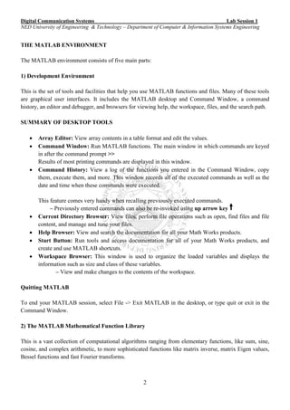
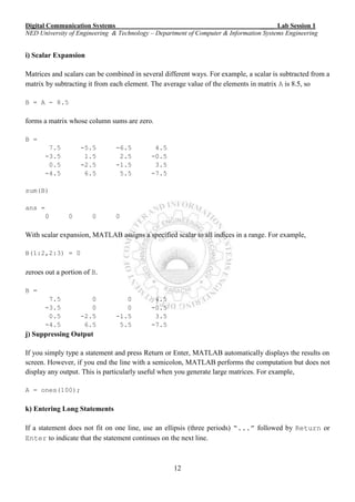
Consider the following vector, x (recall that a vector is simply a matrix with only one row or column)
» x = [1,3,5,7,9,11]
x = 1 3 5 7 9 11
Notice that a row vector is the default. We could have used spaces as the delimiter between
columns
» x = [1 3 5 7 9 11]
x = 1 3 5 7 9 11
There is a faster way to enter matrices or vectors that have a linear pattern. For example, the
following command creates the previous vector
» x = 1:2:11 (here what does ‘2’ indicate? Will be discussed in proceeding lab sessions)
x = 1 3 5 7 9 11
Transposing a row vector yields a column vector ( 'is the transpose command in MATLAB)
» y = x'
y = 1
3
5
7
9
11

8. Digital Communication Systems ____ Lab Session 1
NED University of Engineering & Technology – Department of Computer & Information Systems Engineering
5
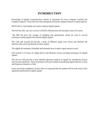
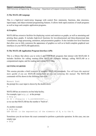
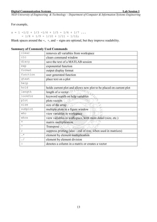
Say that we want to create a vector z, which has elements from 5 to 30, by 5's
» z = 5:5:30
z = 5 10 15 20 25 30
If we wish to suppress printing, we can add a semicolon (;) after any MATLAB command
» z = 5:5:30;
The z vector is generated, but not printed in the command window. We can find the value of the third
element in the z vector, z(3), by typing
» z(3)
ans = 15
(Notice that a new variable, ans, was defined automatically.)
The MATLAB Workspace
We can view the variables currently in the workspace by typing
» who
Your variables are:
ans x y z
leaving 621420 bytes of memory free.
More detail about the size of the matrices can be obtained by typing
» whos
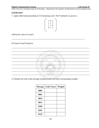
Name Size Total Complex
ans 1 by 1 1 No
x 1 by 6 6 No
y 6 by 1 6 No
z 1 by 6 6 No
Grand total is (19 * 8) = 152 bytes,
leaving 622256 bytes of memory free.
We can also find the size of a matrix or vector by typing
» [m,n]=size(x)
m =1
n =6
where m represents the number of rows and n represents the number of columns.
If we do not put place arguments for the rows and columns, we find
» size(x)
ans = 1 6
Since x is a vector, we can also use the length command
» length(x)
ans = 6

9. Digital Communication Systems ____ Lab Session 1
NED University of Engineering & Technology – Department of Computer & Information Systems Engineering
6
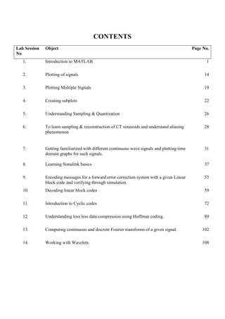
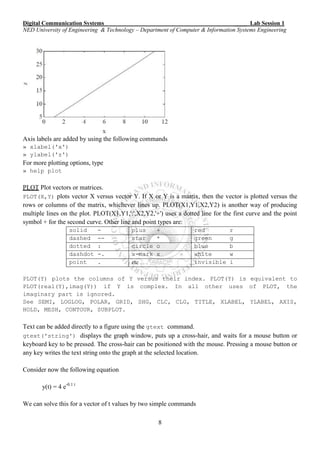
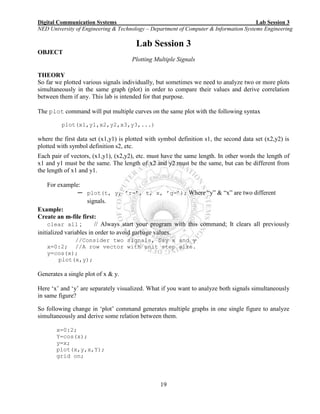
It should be noted that MATLAB is case sensitive with respect to variable names. An X matrix can
coexist with an x matrix. MATLAB is not case sensitive with respect to "built-in" MATLAB functions.
For example, the length command can be upper or lower case
» LENGTH(x)
ans = 6
Notice that we have not named an upper case X variable. See what happens when we try to find the length
of X
» LENGTH(X)
??? Undefined function or variable.
Symbol in question ==> X
Sometimes it is desirable to clear all of the variables in a workspace. This is done by simply typing
» clear
more frequently you may wish to clear a particular variable, such as x
» clear x
You may wish to quit MATLAB but save your variables so you don't have to retype or recalculate them
during your next MATLAB session. To save all of your variables, use
» save file_name
(Saving your variables does not remove them from your workspace; only clear can do that)
You can also save just a few of your variables
» save file_name x y z
To load a set of previously saved variables
» load file_name
b) Complex variables
Both i and j represent the imaginary number, √-1, by default
» i
ans = 0 + 1.0000i
» j
ans = 0 + 1.0000i
» sqrt(-3)
ans = 0 + 1.7321i
Note that these variables (i and j) can be redefined (as the index in a for loop, for example), not
included in your course.
Matrices can be created where some of the elements are complex and the others are real
» a = [sqrt(4), 1;sqrt(-4), -5]

10. Digital Communication Systems ____ Lab Session 1
NED University of Engineering & Technology – Department of Computer & Information Systems Engineering
7
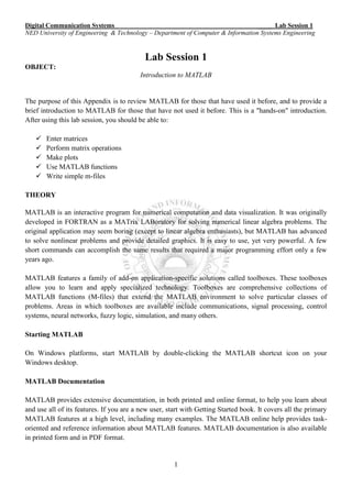
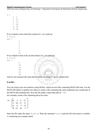
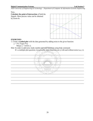
a = 2.0000 1.0000
0 + 2.0000i -5.0000
Recall that the semicolon designates the end of a row.
c) Some Matrix Operations
Matrix multiplication is straight-forward
» b = [1 2 3;4 5 6]
b = 1 2 3
4 5 6
using the a matrix that was generated above:
» c = a*b
c =
6.0000 9.0000 12.0000
-20.0000 + 2.0000i -25.0000 + 4.0000i -30.0000 + 6.0000i
Notice again that MATLAB automatically deals with complex numbers.
Sometimes it is desirable to perform an element by element multiplication. For example, d(i,j) =
b(i,j)*c(i,j) is performed by using the .* command
» d = c.*b
d =
1.0e+02 *0.0600 0.1800 0.3600
-0.8000 + 0.0800i -1.2500 + 0.2000i -1.8000 + 0.3600i
Similarly, element by element division, b(i,j)/c(i,j), can be performed using ./
Other matrix operations include: (i) taking matrix to a power, and (ii) the matrix exponential.
These are operations on a square matrix
» f = a^2
f = 4.0000 + 2.0000i -3.0000
0 - 6.0000i 25.0000 + 2.0000i
» g = expm(a)
g = 7.2232 + 1.8019i 1.0380 + 0.2151i
-0.4302 + 2.0760i -0.0429 + 0.2962i
d) Plotting
For a standard solid line plot, simply type
» plot(x,z)

11. Digital Communication Systems ____ Lab Session 1
NED University of Engineering & Technology – Department of Computer & Information Systems Engineering
8
Axis labels are added by using the following commands
» xlabel('x')
» ylabel('z')
For more plotting options, type
» help plot
PLOT Plot vectors or matrices.
PLOT(X,Y) plots vector X versus vector Y. If X or Y is a matrix, then the vector is plotted versus the
rows or columns of the matrix, whichever lines up. PLOT(X1,Y1,X2,Y2) is another way of producing
multiple lines on the plot. PLOT(X1,Y1,':',X2,Y2,'+') uses a dotted line for the first curve and the point
symbol + for the second curve. Other line and point types are:
solid - plus + red r
dashed -- star * green g
dotted : circle o blue b
dashdot -. x-mark x white w
point . etc . . . invisible i
PLOT(Y) plots the columns of Y versus their index. PLOT(Y) is equivalent to
PLOT(real(Y),imag(Y)) if Y is complex. In all other uses of PLOT, the
imaginary part is ignored.
See SEMI, LOGLOG, POLAR, GRID, SHG, CLC, CLG, TITLE, XLABEL, YLABEL, AXIS,
HOLD, MESH, CONTOUR, SUBPLOT.
Text can be added directly to a figure using the gtext command.
gtext('string') displays the graph window, puts up a cross-hair, and waits for a mouse button or
keyboard key to be pressed. The cross-hair can be positioned with the mouse. Pressing a mouse button or
any key writes the text string onto the graph at the selected location.
Consider now the following equation
y(t) = 4 e-0.1 t
We can solve this for a vector of t values by two simple commands

12. Digital Communication Systems ____ Lab Session 1
NED University of Engineering & Technology – Department of Computer & Information Systems Engineering
9
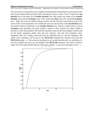
» t = 0:1:50;
» y = 4*exp(-0.1*t);
and we can obtain a plot by typing
» plot(t,y)
Notice that we could shorten the sequence of commands by typing
» plot(t,4*exp(-0.1*t))
we can plot the function y(t) = t e-0.1 t
by using
» y = t.*exp(-0.1*t);
» plot(t,y)
» gtext('hey, this is the peak!')
» xlabel('t')
» ylabel('y')
Further functions related to PLOT will be discussed in proceeding lab sessions
e) More Matrix Stuff
A matrix can be constructed from 2 or more vectors. If we wish to create a matrix v which consists of 2
columns, the first column containing the vector x (in column form) and the second column containing the
vector z (in column form) we can use the following
» v = [x',z']

13. Digital Communication Systems ____ Lab Session 1
NED University of Engineering & Technology – Department of Computer & Information Systems Engineering
10
v =
1 5
3 10
5 15
7 20
9 25
11 30
If we wished to look at the first column of v, we could use
» v(:,1)
ans =
1
3
5
7
9
11
If we wished to look at the second column of v, we could use
» v(:,2)
ans =
5
10
15
20
25
30
And we can construct the same plot as before, by using ('--' gives a dotted line)
f) m-files
You can create your own matrices using M-files, which are text files containing MATLAB code. Use the
MATLAB Editor or another text editor to create a file containing the same statements you would type at
the MATLAB command line. Save the file under a name that ends in “.m”.
For example, create a file containing these five lines.
A = 16 3 2 13
5 10 11 8
9 6 7 12
4 15 14 1
Store the file under the name first.m. Then the statement first reads the file and creates a variable,
A, containing our example matrix.

14. Digital Communication Systems ____ Lab Session 1
NED University of Engineering & Technology – Department of Computer & Information Systems Engineering
11
g) Diary
When preparing homework solutions it is often necessary to save the sequence of commands and output
results in a file to be turned in with the homework. The diary command allows this.
diary file_name causes a copy of all subsequent terminal input and most of the resulting output to be
written on the file named file_name. diary off suspends it. diary on turns it back on. diary, by
itself, toggles the diary state. Diary files may be edited later with a text editor to add comments or remove
mistaken entries.
Often the consultants wish to see a diary file of your session to assist them in troubleshooting your
MATLAB problems.
h) Deleting Rows and Columns
You can delete rows and columns from a matrix using just a pair of square brackets. Start with
X = A;
Then, to delete the second column of X, use
X(:,2) = []
This changes X to
X =
16 2 13
5 11 8
9 7 12
4 14 1
If you delete a single element from a matrix, the result is not a matrix anymore. So, expressions like
X(1,2) = []
will result in an error. However, using a single subscript deletes a single element, or sequence of
elements, and reshapes the remaining elements into a row vector. So
X(2:2:10) = []
results in
X =
16 9 2 7 13 12 1

15. Digital Communication Systems ____ Lab Session 1
NED University of Engineering & Technology – Department of Computer & Information Systems Engineering
12
i) Scalar Expansion
Matrices and scalars can be combined in several different ways. For example, a scalar is subtracted from a
matrix by subtracting it from each element. The average value of the elements in matrix A is 8.5, so
B = A - 8.5
forms a matrix whose column sums are zero.
B =
7.5 -5.5 -6.5 4.5
-3.5 1.5 2.5 -0.5
0.5 -2.5 -1.5 3.5
-4.5 6.5 5.5 -7.5
sum(B)
ans =
0 0 0 0
With scalar expansion, MATLAB assigns a specified scalar to all indices in a range. For example,
B(1:2,2:3) = 0
zeroes out a portion of B.
B =
7.5 0 0 4.5
-3.5 0 0 -0.5
0.5 -2.5 -1.5 3.5
-4.5 6.5 5.5 -7.5
j) Suppressing Output
If you simply type a statement and press Return or Enter, MATLAB automatically displays the results on
screen. However, if you end the line with a semicolon, MATLAB performs the computation but does not
display any output. This is particularly useful when you generate large matrices. For example,
A = ones(100);
k) Entering Long Statements
If a statement does not fit on one line, use an ellipsis (three periods) “...” followed by Return or
Enter to indicate that the statement continues on the next line.

16. Digital Communication Systems ____ Lab Session 1
NED University of Engineering & Technology – Department of Computer & Information Systems Engineering
13
For example,
s = 1 -1/2 + 1/3 -1/4 + 1/5 - 1/6 + 1/7 ...
- 1/8 + 1/9 - 1/10 + 1/11 - 1/12;
Blank spaces around the =, +, and - signs are optional, but they improve readability.
Summary of Commonly Used Commands
clear removes all variables from workspace
clc clears command window
diary save the text of a MATLAB session
exp exponential function
format output display format
function user generated function
gtext place text on a plot
help
hold holds current plot and allows new plot to be placed on current plot
length length of a vector
lookfor keyword search on help variables
plot plots vectors
size size of the array
subplot multiple plots in a figure window
who view variables in workspace
whos view variables in workspace, with more detail (size, etc.)
* matrix multiplication
' Transpose
; suppress printing (also - end of row, when used in matrices)
.* element by element multiplication
./ element by element division
: denotes a column in a matrix or creates a vector

17. Digital Communication Systems ____ Lab Session 2
NED University of Engineering & Technology – Department of Computer & Information Systems Engineering
14
‘3’ Step size
Lab Session 2
OBJECT
Plotting of signals
THEORY:
MATLAB is very useful for making scientific and engineering plots. You can create plots of known,
analytical functions, you can plot data from other sources such as experimental measurements, and you
can analyze data, perhaps by fitting it to a curve, and then plot a comparison. MATLAB also has powerful
built-in routines for drawing contour and three-dimensional surface plots.
Signal’s representation
 A signal in MATLAB is represented by a row vector:
 Examples:
─ x = [2, 3, -5, -3, 1]
─ n = 2:17 = [2, 3, 4, 5, 6, 7, 8, 9, 10, 11, 12, 13, 14, 16, 17]
Default step size is 1
─ n = 2:3:17 = [2, 5, 8, 11, 14, 17]
Plotting in MATLAB
 A vector is plotted against a vector
 lengths of vectors must match
 Two functions
 plot
─ for CT signals
 stem
─ for DT signals
The basic plot command
Two-dimensional line and symbol plots are created with the plot command. In its simplest form plot
takes two arguments
>> plot(xdata,ydata)
where xdata and ydata are vectors containing the data. Note that xdata and ydata must be the same
length and both must be the same type, i.e., both must be either row or column vectors. Additional
arguments to the plot command provide other options including the ability to plot multiple data sets, and a
choice of colors, symbols and line types for the data.
Example
 Plot the following signal
x = 10sin π t
 vector x against vector t
 must decide on vector’s lengths

18. Digital Communication Systems ____ Lab Session 2
NED University of Engineering & Technology – Department of Computer & Information Systems Engineering
15
─ t = [-2:0.002:2]
─ How to generate vector x?
o x = 10 * sin (pi * t)
 plot(t , x)
 plot(t, x) plot([-2:0.002:2], 10 * sin(pi*[-2:0.002:2]))
─ instead of defining “t” & “x” separately, you can directly pass their values/range
 title(‘Example Sinusoid’)
─ to name the plot use “title” command
 xlabel(‘time(sec)’)
 ylabel(‘Amplitude’)
A simple line plot
Here are the MATLAB commands to create a simple plot of y = sin (3*pi*x) from 0 to 2*pi.
>> x = 0:pi/30:2*pi; % x vector, 0 <= x <= 2*pi, increments of pi/30
>> y = sin(3*x); % vector of y values
>> plot(x,y) % create the plot
>> xlabel('x (radians)'); % label the x-axis
>> ylabel('sine function'); % label the y-axis
>> title('sin(3*x)'); % put a title on the plot
The effect of the labeling commands, xlabel, ylabel, and title are indicated by the text and arrows
in the figure below.
CHANGING SYMBOL OR LINE TYPES
The symbol or line type for the data can be changed by passing an optional third argument to the plot
command. For example
>> plot(x,y,'o');
plots data in the x and y vectors using circles drawn in the default color (yellow), and
>> plot(x,y,'r:');
plots data in the x and y vectors by connecting each pair of points with a red dashed line.
Vector on Y-
axis
Vector on X-
axis
to label x-axis and y-axis
Title
X-label
Y-label

19. Digital Communication Systems ____ Lab Session 2
NED University of Engineering & Technology – Department of Computer & Information Systems Engineering
16
The third argument of the plot command is a one, two or three character string of the form 'cs', where 'c' is
a single character indicating the color and 's' is a one or two character string indicating the type of symbol
or line. The color selection is optional. Allowable color and symbols types are summarized in the tables
of lab session#01. Refer to ``help plot'' for further information.
DT Plots
 Plot the DT sequences:
─ x = [2, 3, -1, 5, 4, 2, 3, 4, 6, 1]
─ Stem(x);
─ x = [2, 3, -1, 5, 4, 2, 3, 4, 6, 1]
─ n = -6:3;
─ stem(n, x);
Zero & One Vectors
 zeros(1, 5)
– [0 0 0 0 0]
 ones(1, 5)
– [1 1 1 1 1]
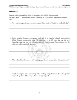
EXERCISES
1. Use Matlab to draw the graph of f (x) = x2
− 2x − 3 on the interval [−1, 3].
_______________________________________________
_______________________________________________
_______________________________________________
_______________________________________________
_______________________________________________
_______________________________________________
_____________________________________________________________________________________
_____________________________________________________________________________________

20. Digital Communication Systems ____ Lab Session 2
NED University of Engineering & Technology – Department of Computer & Information Systems Engineering
17
2. Generate following elementary DT signals:
– Unit Impulse
– Unit Step
– Unit Ramp
– Exponential Sequence
Example:
– Unit Impulse
_______________________________________________
_______________________________________________
_______________________________________________
_______________________________________________
_______________________________________________
_______________________________________________
________________________________________________________________________________
________________________________________________________________________________
– Unit Step
_______________________________________________
_______________________________________________
_______________________________________________
_______________________________________________
_______________________________________________
_______________________________________________
_____________________________________________________________________________________
_____________________________________________________________________________________
– Unit Ramp
_______________________________________________
_______________________________________________
_______________________________________________
_______________________________________________
_______________________________________________
_____________________________________________________________________________________
_____________________________________________________________________________________
n = -5:5;
stem (n, [zeros(1,5) 1 zeros(1,5)])

21. Digital Communication Systems ____ Lab Session 2
NED University of Engineering & Technology – Department of Computer & Information Systems Engineering
18
– Exponential sequence
_______________________________________________
_______________________________________________
_______________________________________________
_______________________________________________
_______________________________________________
_____________________________________________________________________________________
_____________________________________________________________________________________
3. Generate the following signal for -10<n<10
x = (10cosπn)(5cos0.25πn)
_______________________________________________
_______________________________________________
_______________________________________________
_______________________________________________
_______________________________________________
_______________________________________________
________________________________________________________________________________
________________________________________________________________________________

22. Digital Communication Systems Lab Session 3
NED University of Engineering & Technology – Department of Computer & Information Systems Engineering
19
Lab Session 3
OBJECT
Plotting Multiple Signals
THEORY
So far we plotted various signals individually, but sometimes we need to analyze two or more plots
simultaneously in the same graph (plot) in order to compare their values and derive correlation
between them if any. This lab is intended for that purpose.
The plot command will put multiple curves on the same plot with the following syntax
plot(x1,y1,x2,y2,x3,y3,...)
where the first data set (x1,y1) is plotted with symbol definition s1, the second data set (x2,y2) is
plotted with symbol definition s2, etc.
Each pair of vectors, (x1,y1), (x2,y2), etc. must have the same length. In other words the length of
x1 and y1 must be the same. The length of x2 and y2 must be the same, but can be different from
the length of x1 and y1.
For example:
─ plot(t, y, ’r-’, t, x, ’g-’); Where “y” & “x” are two different
signals.
Example:
Create an m-file first:
clear all ; // Always start your program with this command; It clears all previously
initialized variables in order to avoid garbage values.
//Consider two signals, Say x and y
x=0:2; //A row vector with unit step size.
y=cos(x);
plot(x,y);
Generates a single plot of x & y.
Here ‘x’ and ‘y’ are separately visualized. What if you want to analyze both signals simultaneously
in same figure?
So following change in ‘plot’ command generates multiple graphs in one single figure to analyze
simultaneously and derive some relation between them.
x=0:2;
Y=cos(x);
y=x;
plot(x,y,x,Y);
grid on;

23. Digital Communication Systems Lab Session 3
NED University of Engineering & Technology – Department of Computer & Information Systems Engineering
20
Now,
Calculate the point of intersection of both the
Signals. More precise value can be obtained
by Zoom In.
EXERCISES
1. Create a symbol plot with the data generated by adding noise to the given function:
y = 5*x.*exp(-3*x)
Where x = 0:0.01:2;
Hint: In order to add noise study randint and rand functions using help command.
It’s a multiple plot question; two possible input functions are y with and without noise (say y1).
________________________________________________________________________________
________________________________________________________________________________
________________________________________________________________________________
________________________________________________________________________________
________________________________________________________________________________
________________________________________________________________________________
________________________________________________________________________________
________________________________________________________________________________
________________________________________________________________________________
________________________________________________________________________________

24. Digital Communication Systems Lab Session 3
NED University of Engineering & Technology – Department of Computer & Information Systems Engineering
21
2. Sketch the graphs of f (x) = 1/x and g(x) = ln(x − 1) on the interval [2, 5].
________________________________________________________________________________
________________________________________________________________________________
________________________________________________________________________________
________________________________________________________________________________
________________________________________________________________________________

25. Digital Communication Systems Lab Session 4
NED University of Engineering & Technology – Department of Computer & Information Systems Engineering
22
Lab Session 4
OBJECT
Creating subplots
THEORY
Create axes in tiled positions. Subplot divides the current figure into rectangular panes that are
numbered row wise. Each pane contains an axes object. Subsequent plots are output to the current
pane.
h = subplot(m,n,p)breaks the figure window into an m-by-n matrix of small axes, selects
the pth axes object for the current plot, and returns the axes handle. The axes are counted along
the top row of the figure window, then the second row, etc.
For example
 subplot(2, 3, 2)
Upper and Lower Subplots with Titles
To plot income in the top half of a figure and outgo in the bottom half,
income = [3.2 4.1 5.0 5.6];
outgo = [2.5 4.0 3.35 4.9];
subplot(2,1,1); plot(income)
title('Income')
subplot(2,1,2); plot(outgo)
title('Outgo')
2 rows Plot #; plot in which graph is desired3 cols
1 2 3
4 5 6
2Rows
3 Columns

26. Digital Communication Systems Lab Session 4
NED University of Engineering & Technology – Department of Computer & Information Systems Engineering
23
Example:
Create a file called 'exa1_2.m'. In this file put the following:
t = [0 1 2 3 4]; %basic plotting
plot(t) %pointwise plotting with default blue color
and
%‘-‘which joins all the points
axis([0 8 0 8]);
%-------ADD-------
plot(t, 2*t, 'r+'); %add hold on also put this before the axis
%command
%-------ADD-------
figure; %use this command to open another plot
%on a separate window
x = pi*[-24:24]/24; %x-axis does not show true points
plot(x,sin(x));
xlabel('radians'); %x-label
ylabel('sin value'); %y-label
title( 'dummy' ); %title
%-------ADD-------
figure; %multiple functions in separate graphs
subplot( 2,2,2 );
axis square
subplot( 2,2,4 );
axis square
subplot( 2,2,[1 3]); %try square axis

27. Digital Communication Systems Lab Session 4
NED University of Engineering & Technology – Department of Computer & Information Systems Engineering
24
EXERCISES
1. Write a sequence of MATLAB commands in the space below to plot the discrete time sinusoid
x (n) = cosωn (-5 < n < 5) for the following values of angular frequency. You must divide your
figure into 6 subplots. What’s the conclusion?
 ω = 0.10π
 ω = 0.25π
 ω = π
 ω = 1.25π
 ω = 1.50π
 ω = 2π
________________________________________________________________________________
________________________________________________________________________________
________________________________________________________________________________
________________________________________________________________________________
________________________________________________________________________________
________________________________________________________________________________
________________________________________________________________________________
________________________________________________________________________________
________________________________________________________________________________
________________________________________________________________________________
________________________________________________________________________________
________________________________________________________________________________
________________________________________________________________________________
________________________________________________________________________________
________________________________________________________________________________
________________________________________________________________________________
________________________________________________________________________________
________________________________________________________________________________
________________________________________________________________________________
________________________________________________________________________________

28. Digital Communication Systems Lab Session 4
NED University of Engineering & Technology – Department of Computer & Information Systems Engineering
25
2. Ten sources (users) are generating data in bits randomly. Each user is generating 16 bits/message
and each message contains four symbols. The data is fed into a block which converts each symbol
into its decimal representation. Perform the following:
 Compute the mean and the maximum values of the decimal representation of these
messages for individual users.
 Display the matrix of messages in both bits and decimals form.
 Display the values of mean and maximum for all users.
 Plot both results (i.e. one for maximum values and the other for mean values) in the same
window (i.e. figure) up and down.
 Make your program simple and as dynamic as possible.
________________________________________________________________________________
________________________________________________________________________________
________________________________________________________________________________
________________________________________________________________________________
________________________________________________________________________________
________________________________________________________________________________
________________________________________________________________________________
________________________________________________________________________________
________________________________________________________________________________
________________________________________________________________________________

29. Digital Communication Systems Lab Session 5
NED University of Engineering & Technology – Department of Computer & Information Systems Engineering
26
Lab Session 5
OBJECT
Understanding Sampling & Quantization
THEORY:
Sampling:
An analog signal is characterized by the fact that its attributes (like: amplitude, frequency and
phase) can take any value over a continuous range. On the other hand, digital signals can take only
discrete and finite values. One can convert an analog signal to a digital signal by sampling and
quantizing (collectively called analog-to-digital conversion, or ADC). It is typically more efficient
to process the resulting discrete signals by digital signal processors. The processed signals are then
converted back into analog signals using a reconstruction or interpolation operation (called digital-
to-analog conversion, or DAC).
To sample a continuous-time signal )(tx is to represent )(tx at a discrete number of points, SnTt  ,
where ST is the sampling period. The sampling theorem states that a band-limited signal )(tx with
bandwidth W can be reconstructed from its sample values )()( SnTxnx  if the sampling
frequency SS Tf /1 is greater than twice the bandwidth W of )(tx . Otherwise, aliasing would
result in )(tx . The minimum sampling rate of 2W for an analog band-limited signal is called the
Nyquist rate.
Quantization:
In order to process the sampled signal digitally, the sample values have to be quantized to a finite
number of levels, and each value can then be represented by a string of bits. For example, if the
signal is quantized to N different levels, then log2(N) bits per sample are required. Notice that to
quantize a sample value is to round it to the nearest point among a finite set of permissible values.
Therefore, a distortion will inevitably occur. This is called quantization noise (or error).
Quantization can be classified as uniform and non-uniform. In the case of uniform quantization, the
quantization regions are chosen to have equal length. However, in non-uniform quantization,
regions of various lengths are allowed. Non-uniform quantization can be implemented through
compression-expansion of the signal, and this is commonly used (as in telephony) to maintain a
uniform signal-to-quantization noise ratio over the full dynamic range of the signal (refer to your
textbook for more details).

30. Digital Communication Systems Lab Session 5
NED University of Engineering & Technology – Department of Computer & Information Systems Engineering
27
EXERCISES
Generate a time vector t from -0.5 to 0.5 with a step size of 0.001. Implement the
function
pt
etx
/
)(

 where p=0.1. In order to simulate an A/D converter, perform the following
tasks:
1. Plot x and its magnitude spectrum in a two-panel figure window. What is the bandwidth of x?
________________________________________________________________________________
________________________________________________________________________________
________________________________________________________________________________
2. Set the sampling frequency to twice the bandwidth of the signal x (which is approximately
25Hz). Generate a rectangular pulse train starting at -0.5 to 0.5 where the step size is 1/
(sampling frequency) and with a duration of 0.0001. In a two-panel figure window, plot the
pulse train and its magnitude spectrum.
________________________________________________________________________________
________________________________________________________________________________
________________________________________________________________________________
3. What is the relation between the time and frequency domain representation of the pulse train?
________________________________________________________________________________
________________________________________________________________________________
________________________________________________________________________________
4. Sample x using the pulse train and plot the resulting sampled version of x. Also, plot its
magnitude spectrum. What can you observe from both plots?
________________________________________________________________________________
________________________________________________________________________________

31. Digital Communication Systems Lab Session 6
NED University of Engineering & Technology – Department of Computer & Information Systems Engineering
28
Lab Session 6
OBJECT
To learn sampling & reconstruction of CT sinusoids and understand aliasing phenomenon
THEORY:
Sampling Principle
A CT sinusoid containing a maximum frequency of Fmax must be sampled at a sampling rate
Fs > 2Fmax (Nyquist Rate) to avoid aliasing.
If sampling rate is greater than Nyquist Rate, then CT sinusoid can be uniquely recovered from its
DT version.
Alias Frequency
Analog frequencies separated by integral multiple of a given sampling rate are alias of each other–
Any CT sinusoid of frequency Fk when sampled at the sampling rate Fs will result in the same DT
sinusoid as does the CT sinusoid of frequency F0 sampled at Fs, where:
Fk = F0 + kFs; k = ±1, ±2, ±3 . . .
Example:
Assume two CT sinusoidal signals
– x1(t) = cos(2p t)
• F1 = 1 Hz
– x2(t) = cos(6p t)
• F2 = 3 Hz
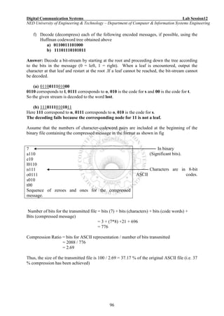
These signals can be plotted using the MATLAB code shown:
t = -2:0.005:2;
x1 = cos(2*pi*t);
x2 = cos(6*pi*t);
subplot(3,2,1),plot(t, x1);
axis([-2 2 -1 1]); grid on;
xlabel('t'), ylabel('cos2pit');
subplot(3,2,2), plot(t, x2);
axis([-2 2 -1 1]); grid on;
xlabel('t'), ylabel('cos6pit');
The Axis Command
axis ([xmin xmax ymin ymax]);
This command is used to adjust the axis settings of plots.
Discretizing the Signals
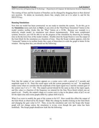
Assume sampling rate = 2 samples/s
You’ll notice a slight change in how we sample signals using MATLAB than what we do using
paper-pencil
n = -2:1/2:2;
• Note that sampling interval appears as step size for the vector

32. Digital Communication Systems Lab Session 6
NED University of Engineering & Technology – Department of Computer & Information Systems Engineering
29
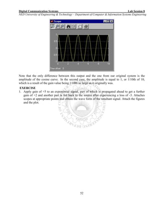
Plotting DT Sinusoid
x1n = cos(2*pi*[-2:1/2:2]);
• Should we plot it against n?
• NO!
Because this will depict sampled signal incorrectly.
Generate another vector from n as follows:
k = -2:length(n)-3;
subplot(3,2,3),
stem(k, x1n);
axis([-2 length(n)-3 -1 1]);
grid on;
xlabel('n'),
ylabel('cospin');
subplot(3,2,4),
stem(k, x2n);
axis([-2 length(n)-3 -1 1]);
grid on;
xlabel('n'),
ylabel('cos3pin');
Reconstruction
• D/A conversion
– performed using interpolation
• There are various approaches to interpolation but here we are using
– Cubic Spline Interpolation
 invoked by spline(n, xn, t)

33. Digital Communication Systems Lab Session 6
NED University of Engineering & Technology – Department of Computer & Information Systems Engineering
30
EXERCISES
X (t) = 50 cos300πt – 100 cos250πt
1. What’s the Nyquist rate?
________________________________________________________________________________
________________________________________________________________________________
________________________________________________________________________________
2. Let the signal be sample at 200 Hz. Find the frequencies in the resulting DT sinusoid.
________________________________________________________________________________
________________________________________________________________________________
________________________________________________________________________________
3. If the DT signal obtained in part (b) is passed through an ideal D/A converter operating at
200 samples per second, what the reconstructed signal?
________________________________________________________________________________
________________________________________________________________________________
________________________________________________________________________________
4. Determine the fundamental period of the DT sinusoid obtained in part (b)
________________________________________________________________________________
________________________________________________________________________________
________________________________________________________________________________
5. Perform the above conversion (from CT to DT and extract CT back from the derived DT
signal) using Matlab commands.
________________________________________________________________________________
________________________________________________________________________________
________________________________________________________________________________
6. Was the original signal reconstructed?
________________________________________________________________________________
________________________________________________________________________________

34. Digital Communication Systems Lab Session 7
NED University of Engineering & Technology – Department of Computer & Information Systems Engineering
31
Lab Session 7
OBJECT
Getting familiarized with different continuous wave signals and plotting time domain graphs for
such signals.
THEORY
A signal is a form in which data is transmitted. It describes the behavior of data. Mathematically
represented by a dependent variable (e.g. x(t)) and independent variable (in this case t).
Special type of signal is the sinusoid wave which is a combination of sine and cosine waves. These
signals are easy to visualize, generate and process. Any signal could be represented by the sum of
these sinusoidal waves.
There are three parameters mainly that describe a signal: Amplitude, frequency and phase.
Amplitude describes the strength or intensity of the signal at a given time. Frequency means the
number of cycle or repetition per second. This definition is only valid for periodic signals since
periodic signals repeat themselves everyT second (known as the period time duration). For non-
periodic signals, these are converted or represented by periodic sinusoid signals. Each sinusoid
signal represents a single frequency.
A typical sinusoid signal is given by: )2sin()(   ftAtx ,where  represents the phase of the
signal which describes the position of the signal w.r.t time. A is the amplitude of the signal which
describes the intensity of the signal at a given time. 0f is the frequency which is the number of
cycles per second.
Signal classifications:
1. Periodic and non-periodic:
Periodic signals are those signals that repeat themselves over a period of time known as the period
of the signal (e.g. sine function) and given by:
00 /1 fT  and )()( 0Ttxtx 
Aperiodic signal is one which does not repeat itself. E.g. exponential signals.
A sinusoidal wave has only one frequency which represents the cycles/sec.Other periodic signals
might have more than one frequency and 0f is known as the fundamental frequency which actually
represents the cycles/sec for that signal. All other frequencies usually are integer multiple of the
fundamental frequency.
1)( 2
 ttx

35. Digital Communication Systems Lab Session 7
NED University of Engineering & Technology – Department of Computer & Information Systems Engineering
32
2. Random and deterministic:
Deterministic signals: are those signals which we can construct using a mathematical relation, table
lookup and by other means.
Random signals: those signals which have some level of uncertainty. We can estimate theses signal
by statistical and probabilistic means.
3. Power and Energy signals:
A signal is known as energy signal if it has finite energy but zero average power
E.g. deterministic and aperiodic signals.
A signal is known as power signal if it has finite average power but infinite energy. e.g. random
and periodic signals.
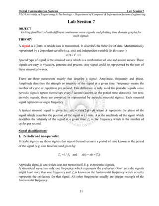
Simple operations on signals:
1. scaling )()( tmxtg  where m is a scalar quantity. (Amplification and attenuation)
2. Addition. (e.g. FT concept).
3. Modulation. tfAtxtg c2cos)()(  where cff 0
4. Delay and advancement of a signal. )( 0ttx  and )( 0ttx 
5. Time reversal )( tx  .
Continuous signals in MATLAB:
There is no realization of continuous signals in MATLAB. A continuous signal is represented by
discrete points chosen at discrete points.
Examples:
Sinusoidal signals:
A=[10 6 4]; %vary the amplitude. make them equal
p=[0 pi/2 pi]; %vary the phase.
f=40; %frequency can vary and T accordingly.
n=1; %change the cycle number to display.
t=[n*(-0.025):0.001:n*(0.025)]; %choose the range according to the
%number of cycles n. You can display
%only positive t values.
for k=1:3
x{k} = A(k).*sin((2*pi*n*f*t)+p(k));
plot(t,x{k})
hold on
end
%Additional plot for all signals with different colors
figure
plot(t,x{1},t,x{2},t,x{3})
clear all

36. Digital Communication Systems Lab Session 7
NED University of Engineering & Technology – Department of Computer & Information Systems Engineering
33
Signum function:
t=[-10:0.001:10]; %time range. try to increase and decrease range
y = sign(t); %signum function
plot(t,y);
sinc function:
sinc computes the sinc function of an input vector or array, where the sinc function is:
)(sin xc 1 for 0t
x
x

 )sin(
 otherwise.
A=3; %vary
p=40;
t=[(-0.05):0.001:(0.05)]; %only positive t values.
y = A.*sinc(2*p*t); %sinc punction
plot(t,y);
figure
x = abs(A.*sinc(2*p*t)); %magnitude sinc punction
plot(t,x);
Square wave (single period):
A=3; %vary
f0=1/10; %frequency of the square wave
T0=1/f0; %duration of single pulse
t=[-T0/2:0.01:T0/2]; %range is fixed for one symbol duration
%implementation of square wave.
for k=1:length(t)
if (abs(t)<=T0)
x(k)=A;
else
x(k)=0;
end
end
%to connect the last point to zero to give a rectangular shape
%also experiment with the plot properties to see the wave
y=[0,x,0];
t=[-T0/2,t,T0/2];
plot(t,y)
clear all

37. Digital Communication Systems Lab Session 7
NED University of Engineering & Technology – Department of Computer & Information Systems Engineering
34
Another way of implementing signals:
x = sym('x') creates a symbolic object of variable x. So x is actually a symbol variable. Another
way to declare a variable to be a symbol object by writing: syms x y So we have two symbols
with the name x and y.
Now x or y can contain any mathematical expression. Try y=x+1
Implement the following:
syms x y z
x
y=z+x+1
x=sym(1/2)
y
y=z+x+1
x=sym(1:5);
y=z+x+1
z=sym(2)
y=z+x+1
Impulse function or (Dirac delta):
Try dirac(2),dirac(-5),dirac(0). This is equivalent to )(t .
Try:
t=[-10:0.1:10]; %try decreasing the increment.
x=dirac(t);
plot(t,x)
clear all
Integration of a function:
syms x y z
y=x+1;
z=int(y,x) %means integrate y with respect to x
m=int(y,x,0,1) %means integrate y with respect to x
%with the limit from o to 1
clear all
%or try
syms x y z
y=sin(x)
z=int(y,x)
m=int(y,x,-inf,inf)
Signal Operations:
%The following progran is going to perform: Scaling,Addition,Modulation

38. Digital Communication Systems Lab Session 7
NED University of Engineering & Technology – Department of Computer & Information Systems Engineering
35
%and time shift is left as excercise.
%Scaling
t = [-2:0.001:2];
s = t;
s1 = 5*t;
plot (t,s)
hold on
plot (t,s1,'r')
x = sin(2*pi*0.5*t);
figure;
plot (t,x)
hold on
plot (t,5*x,'r')
hold on
plot (t,0.2*x,'g')
%Adding
p1 = s1 + x ;
p2 = x + 2;
figure;
plot(t,p1)
hold on
plot(t,p2)
%modulation
y = 20*cos (2*pi*3*t);
z = s .* y;
figure;
plot(t,z,'m')
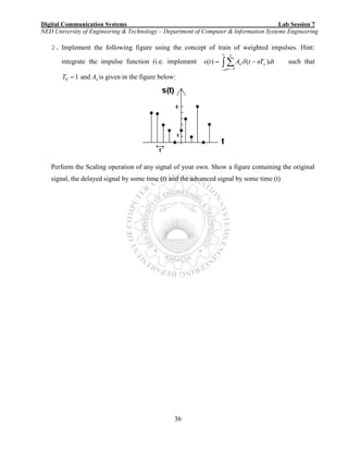
EXERCISES
1. Only for positive values of t , if bit 1 is represented by a square wave with +5 Volts and bit
0 with -5 Volts, and if the duration of a bit is 1 second, then plot a time graph for the
following sequence: 1011010001

39. Digital Communication Systems Lab Session 7
NED University of Engineering & Technology – Department of Computer & Information Systems Engineering
36
2. Implement the following figure using the concept of train of weighted impulses. Hint:
integrate the impulse function (i.e. implement dtTntAts o
n
n )()(
5
5
 

 
  such that
10 T and nA is given in the figure below:
Perform the Scaling operation of any signal of your own. Show a figure containing the original
signal, the delayed signal by some time (t) and the advanced signal by some time (t)

40. Digital Communication Systems Lab Session 8
NED University of Engineering & Technology – Department of Computer & Information Systems Engineering
37
Lab Session 8
OBJECT
Learning Simulink basics
THEORY
The objective of this practical is to acquaint the student with the basic tools needed to use the
SIMULINK package Computing System (CS). SIMULINK is an extension to MATLAB which
uses an icon-driven interface for the construction of a block diagram representation of a process. A
block diagram is simply a graphical representation of a process (which is composed of an input, the
system, and an output).
Typically, the MATLAB m-file is used to solve sets of linear and nonlinear ordinary differential
equations. The “traditional” numerical methods approach is used, e.g. supply the equations to be
solved in a function file, and use a general purpose equation solver (linear or nonlinear algebraic,
linear or nonlinear differential equation, etc.) which “calls” the supplied function file to obtain the
solution. One of the reasons why MATLAB is relatively easy to use is that the “equation solvers”
are supplied for us, and we access these through a command line interface (CLI) (aka the
MATLAB prompt, >>).
However, SIMULINK uses a graphical user interface (GUI) for solving process simulations.
Instead of writing MATLAB code, we simply connect the necessary “icons” together to construct
the block diagram. The “icons” represent possible inputs to the system, parts of the systems, or
outputs of the system. SIMULINK allows the user to easily simulate systems of linear and
nonlinear ordinary differential equations. A good background in matrix algebra and lumped
parameter systems as well as an understanding of MATLAB is required, and we highly recommend
that the student thoroughly reads and works through this tutorial. Many of the features of
SIMULINK are user-friendly due to the icon-driven interface, yet it is important to spend some
time experimenting with SIMULINK and its many features. Dynamic simulation packages (such as
MATLAB, SIMULINK, etc.) are being used more and more frequently in the chemical process
industries for process simulation and control system design.

41. Digital Communication Systems Lab Session 8
NED University of Engineering & Technology – Department of Computer & Information Systems Engineering
38
GETTING STARTED IN SIMULINK
SIMULINK is an icon-driven state of the art dynamic simulation package that allows the user to
specify a block diagram representation of a dynamic process. Assorted sections of the block
diagram are represented by icons which are available via various "windows" that the user opens
(through double clicking on the icon). The block diagram is composed of icons representing
different sections of the process (inputs, state-space models, transfer functions, outputs, etc.) and
connections between the icons (which are made by "drawing" a line connecting the icons). Once the
block diagram is "built", one has to specify the parameters in the various blocks, for example the
gain of a transfer function. Once these parameters are specified, then the user has to set the
integration method (of the dynamic equations), stepsize, start and end times of the integration, etc.
in the simulation menu of the block diagram window.
In order to use SIMULINK the student must ``start'' a MATLAB session (click on the MATLAB
button). Once MATLAB has started up, type Simulink (SMALL LETTERS!) at the MATLAB
prompt (>>) followed by a carriage return (press the return key). A SIMULINK window should
appear shortly, with the following icons: Sources, Sinks, Discrete, Linear, Nonlinear, Connections,
Extras. Next, go to the file menu in this window and choose New in order to begin building the
block diagram representation of the system of interest.
BLOCK DIAGRAM CONSTRUCTION
As mentioned previously, the block diagram representation of the system is made up of various type
of icons. Basically, one has to specify the model of the system (state space, discrete, transfer
functions, nonlinear ODE's, etc), the input (source) to the system, and where the output (sink) of the
simulation of the system will go. Open up the Sources, Sinks, and Linear windows by clicking on
the appropriate icons. Note the different types of sources (step function, sinusoidal, white noise,
etc.), sinks (scope, file, workspace), and linear systems (transfer function, state space model, etc.).
For example, you may be interested in simulating a step input to a first-order transfer function in the
Laplace domain and viewing the result graphically in MATLAB. To do this, you would "drag" a
step function icon from the Sources window, a transfer function icon from the Linear window,
two to workspace icons from the Sinks window, and a clock icon from the Source window to the
blank block diagram window.

42. Digital Communication Systems Lab Session 8
NED University of Engineering & Technology – Department of Computer & Information Systems Engineering
39
The next step is to connect these icons together by drawing lines connecting the icons using the left-
most mouse button (hold the button down and drag the mouse to draw a line). Connect the step
function icon to the input of the transfer function icon, then connect the output of the transfer
function icon to first to workspace icon. Then, connect the clock icon to the second to workspace
icon. ``Open'' the icons (by double clicking on them with the left-most mouse button) and set the
values of the various parameters; for example the step size and step time in the step function icon,
the transfer function coefficients in the transfer function icon, and the variable names in the to
workspace icons (generally, the clock variable is denote as time, whereas the output variable is
denoted y). Select the parameter field from the simulation menu (in the block diagram window) and
set the proper integration details (min and max stepsizes, start and stop integration times,
integration code, etc.). Finally, select start from the simulation menu to start the simulation. The
output of the simulation will be sent to the MATLAB command line interface (CLI) (aka the
MATLAB prompt, >>). The result can be plotted as one would normally plot ( e.g. plot(time,y) ),
since the variables time and y are now defined in the MATLAB workspace. The result is shown in
Figure, for a first-order transfer function with a time constant = 2, and a unit step input at time = 1.

43. Digital Communication Systems Lab Session 8
NED University of Engineering & Technology – Department of Computer & Information Systems Engineering
40
GENERAL SIMULINK TIPS
The following are general tips and should be used often.
1. In order to save your work, select Save from the file menu and give the file that you want to
save a name (or choose an old name if you are ``writing over'' an old version), and click the
ok button (using the left-most mouse button). Realize that you have a choice of the ``folder''
that the file is saved in.
2. The PID Controller block parameters are entered in as: , , .
3. The following transfer function (in the Laplace domain)
is entered into the transfer function icon by double clicking on the transfer function icon
and entering the numerator and denominator polynomial coefficients. The numerator
coefficients would be entered as [2 1] and the denominator coefficients are entered as
[10 5 1].
4. The following state-space A matrix
is entered into the state space icon as [1.0 -2.8;-3.1 0.2].
5. The results of a simulation can be sent to the MATLAB window by the use of the to
workspace icon from the Sinks window. Open the to workspace icon and select the
variable name that you want the results stored in the MATLAB workspace.
6. If your simulation has n state (or output) variables and you want to save them as different
names, then you have to use a special connection called a Demux (as in demultiplexer) icon
which is found in the Connections window. Basically, it takes a vector input and converts it
into several scalar lines. You can set the number of outputs (scalar lines) by double clicking
on the icon and changing the number of outputs. A Mux icon takes several scalar inputs and
multiplexes those in a vector (useful sometimes in transferring the results of a simulation to
the MATLAB workspace, for example).
7. You can generate white (random) noise by selecting the white noise icon from the Source
window.

44. Digital Communication Systems Lab Session 8
NED University of Engineering & Technology – Department of Computer & Information Systems Engineering
41
8. You can use a Gain icon from the Linear window if you need to multiple a signal by a
constant number.
9. You can convert back to physical variables after a state-space or transfer function simulation
by using the Constant icon from the Sources window and a Sum icon from the Sources
window. To do this for a scalar output signal, just enter the value of the steady-state into the
Constant icon and add this to the scalar output using the Sum icon. For a vector output, you
must first "break-up" the vector into scalar outputs using the Demux icon and then add the
steady-state value to each scalar output.
10. The signs of the Sum icon may be changed to negative (in order to subtract) by double
clicking on the Sum icon and changing the sign from a positive to a negative sign. The
number of inputs to the Sum icon may be changed by double clicking on the Sum icon and
setting the number of inputs in the window.
11. Make sure to set the integration parameters in the simulation menu. In particular, the default
minimum and maximum step sizes must be changed (they should be around 1/100 to 1/10 of
the dominant (slowest) time constant of your system).
12. Parameters can be "passed" to SIMULINK from the MATLAB window by using the
parameter in a SIMULINK block or parameter box and defining the parameter in the
MATLAB window. For example, say that one wants to run the simulation with many
different process gains, then in the transfer function icon the gain (in the numerator) can be
given the symbol k (or any symbol) and then at the MATLAB prompt define k = 1.0. Run
the simulation, then at the MATLAB prompt redefine k = 1.5, etc. This is very useful if the
student wants to study the influence of a parameter on the dynamic behavior of a process
(important in determining stability).
13. In order to print the block diagram, first save the block diagram. Then, at the MATLAB
prompt, type:
print -sname-of-simulink-block
where name-of-simulink-block is the name that you saved the block diagram under. For
example, if you saved the block diagram as homework1.m, then you would type:
print -shomework1
14. Time delays (deadtimes) can be simulated in SIMULINK easily by using a transport delay
icon from the Nonlinear window. Double click on the transport delay icon to set the value

45. Digital Communication Systems Lab Session 8
NED University of Engineering & Technology – Department of Computer & Information Systems Engineering
42
of the deadtime.
15. Nonlinear systems can be simulated in SIMULINK using an s-function icon from the
Extras window. The nonlinear ordinary differential equations must be specified in an m-file,
and the name of this m-file is specified in the s-function by the user. We will generally
supply the student with the m-file containing the nonlinear ordinary differential equations.
TABLE OF SIMULINK BLOCKS

46. Digital Communication Systems Lab Session 8
NED University of Engineering & Technology – Department of Computer & Information Systems Engineering
43

47. Digital Communication Systems Lab Session 8
NED University of Engineering & Technology – Department of Computer & Information Systems Engineering
44
Starting Simulink
Simulink is started from the MATLAB command prompt by entering the following command:
simulink
Alternatively, you can click on the "Simulink Library Browser" button at the top of the MATLAB
command window as shown below:
The Simulink Library Browser window should now appear on the screen. Most of the blocks
needed for modeling basic systems can be found in the subfolders of the main "Simulink" folder
(opened by clicking on the "+" in front of "Simulink").
Basic Elements
There are two major classes of elements in Simulink: blocks and lines. Blocks are used to generate,
modify, combine, output, and display signals. Lines are used to transfer signals from one block to
another.

48. Digital Communication Systems Lab Session 8
NED University of Engineering & Technology – Department of Computer & Information Systems Engineering
45
Blocks
The subfolders underneath the "Simulink" folder indicate the general classes of blocks available for
us to use:
 Continuous: Linear, continuous-time system elements (integrators, transfer functions, state-
space models, etc.)
 Discrete: Linear, discrete-time system elements (integrators, transfer functions, state-space
models, etc.)
 Functions & Tables: User-defined functions and tables for interpolating function values
 Math: Mathematical operators (sum, gain, dot product, etc.)
 Nonlinear: Nonlinear operators (coulomb/viscous friction, switches, relays, etc.)
 Signals & Systems: Blocks for controlling/monitoring signal(s) and for creating subsystems
 Sinks: Used to output or display signals (displays, scopes, graphs, etc.)
 Sources: Used to generate various signals (step, ramp, sinusoidal, etc.)
Blocks have zero to several input terminals and zero to several output terminals. Unused input
terminals are indicated by a small open triangle. Unused output terminals are indicated by a small
triangular point. The block shown below has an unused input terminal on the left and an unused
output terminal on the right.
Lines
Lines transmit signals in the direction indicated by the arrow. Lines must always transmit signals
from the output terminal of one block to the input terminal of another block. One exception to this
is that a line can tap off of another line. This sends the original signal to each of two (or more)
destination blocks, as shown below:

49. Digital Communication Systems Lab Session 8
NED University of Engineering & Technology – Department of Computer & Information Systems Engineering
46
Lines can never inject a signal into another line; lines must be combined through the use of a block
such as a summing junction.
A signal can be either a scalar signal or a vector signal. For Single-Input, Single-Output systems,
scalar signals are generally used. For Multi-Input, Multi-Output systems, vector signals are often
used, consisting of two or more scalar signals. The lines used to transmit scalar and vector signals
are identical. The type of signal carried by a line is determined by the blocks on either end of the
line.
Building a System
To demonstrate how a system is represented using Simulink, we will build the block diagram for a
simple model consisting of a sinusoidal input multiplied by a constant gain, which is shown below:
This model will consist of three blocks: Sine Wave, Gain, and Scope. The Sine Wave is a Source
Block from which a sinusoidal input signal originates. This signal is transferred through a line in
the direction indicated by the arrow to the Gain Math Block. The Gain block modifies its input
signal (multiplies it by a constant value) and outputs a new signal through a line to the Scope
block. The Scope is a Sink Block used to display a signal (much like an oscilloscope).
We begin building our system by bringing up a new model window in which to create the block
diagram. This is done by clicking on the "New Model" button in the toolbar of the Simulink
Library Browser (looks like a blank page).
Building the system model is then accomplished through a series of steps:
1. The necessary blocks are gathered from the Library Browser and placed in the model
window.
2. The parameters of the blocks are then modified to correspond with the system we are
modelling.
3. Finally, the blocks are connected with lines to complete the model.

50. Digital Communication Systems Lab Session 8
NED University of Engineering & Technology – Department of Computer & Information Systems Engineering
47
Each of these steps will be explained in detail using our example system. Once a system is built,
simulations are run to analyze its behavior.
Gathering Blocks
Each of the blocks we will use in our example model will be taken from the Simulink Library
Browser. To place the Sine Wave block into the model window, follow these steps:
1. Click on the "+" in front of "Sources" (this is a subfolder beneath the "Simulink" folder) to
display the various source blocks available for us to use.
2. Scroll down until you see the "Sine Wave" block. Clicking on this will display a short
explanation of what that block does in the space below the folder list:
3. To insert a Sine Wave block into your model window, click on it in the Library Browser and
drag the block into your workspace.
The same method can be used to place the Gain and Scope blocks in the model window. The
"Gain" block can be found in the "Math" subfolder and the "Scope" block is located in the "Sink"
subfolder. Arrange the three blocks in the workspace (done by selecting and dragging an individual
block to a new location) so that they look similar to the following:

51. Digital Communication Systems Lab Session 8
NED University of Engineering & Technology – Department of Computer & Information Systems Engineering
48
Modifying the Blocks
Simulink allows us to modify the blocks in our model so that they accurately reflect the
characteristics of the system we are analyzing. For example, we can modify the Sine Wave block
by double-clicking on it. Doing so will cause the following window to appear:
This window allows us to adjust the amplitude, frequency, and phase shift of the sinusoidal input.
The "Sample time" value indicates the time interval between successive readings of the signal.
Setting this value to 0 indicates the signal is sampled continuously.
Let us assume that our system's sinusoidal input has:
 Amplitude = 2
 Frequency = pi
 Phase = pi/2

52. Digital Communication Systems Lab Session 8
NED University of Engineering & Technology – Department of Computer & Information Systems Engineering
49
Enter these values into the appropriate fields (leave the "Sample time" set to 0) and click "OK" to
accept them and exit the window. Note that the frequency and phase for our system contain 'pi'
(3.1415...). These values can be entered into Simulink just as they have been shown.
Next, we modify the Gain block by double-clicking on it in the model window. The following
window will then appear:
Note that Simulink gives a brief explanation of the block's function in the top portion of this
window. In the case of the Gain block, the signal input to the block (u) is multiplied by a constant
(k) to create the block's output signal (y). Changing the "Gain" parameter in this window changes
the value of k.
For our system, we will let k = 5. Enter this value in the "Gain" field, and click "OK" to close the
window.
The Scope block simply plots its input signal as a function of time, and thus there are no system
parameters that we can change for it. We will look at the Scope block in more detail after we have
run our simulation.
Connecting the Blocks
For a block diagram to accurately reflect the system we are modeling, the Simulink blocks must be
properly connected. In our example system, the signal output by the Sine Wave block is
transmitted to the Gain block. The Gain block amplifies this signal and outputs its new value to the
Scope block, which graphs the signal as a function of time. Thus, we need to draw lines from the
output of the Sine Wave block to the input of the Gain block, and from the output of the Gain block
to the input of the Scope block.
Lines are drawn by dragging the mouse from where a signal starts (output terminal of a block) to
where it ends (input terminal of another block). When drawing lines, it is important to make sure
that the signal reaches each of its intended terminals. Simulink will turn the mouse pointer into a
crosshair when it is close enough to an output terminal to begin drawing a line, and the pointer will
change into a double crosshair when it is close enough to snap to an input terminal. A signal is
properly connected if its arrowhead is filled in. If the arrowhead is open, it means the signal is not
connected to both blocks. To fix an open signal, you can treat the open arrowhead as an output
terminal and continue drawing the line to an input terminal in the same manner as explained before.

53. Digital Communication Systems Lab Session 8
NED University of Engineering & Technology – Department of Computer & Information Systems Engineering
50
Properly Connected Signal Open Signal
When drawing lines, you do not need to worry about the path you follow. The lines will route
themselves automatically. Once blocks are connected, they can be repositioned for a neater
appearance. This is done by clicking on and dragging each block to its desired location (signals
will stay properly connected and will re-route themselves).
After drawing in the lines and repositioning the blocks, the example system model should look like:
In some models, it will be necessary to branch a signal so that it is transmitted to two or more
different input terminals. This is done by first placing the mouse cursor at the location where the
signal is to branch. Then, using either the CTRL key in conjunction with the left mouse button or
just the right mouse button, drag the new line to its intended destination. This method was used to
construct the branch in the Sine Wave output signal shown below:

54. Digital Communication Systems Lab Session 8
NED University of Engineering & Technology – Department of Computer & Information Systems Engineering
51
The routing of lines and the location of branches can be changed by dragging them to their desired
new position. To delete an incorrectly drawn line, simply click on it to select it, and hit the
DELETE key.
Running Simulations
Now that our model has been constructed, we are ready to simulate the system. To do this, go to
the Simulation menu and click on Start, or just click on the "Start/Pause Simulation" button in the
model window toolbar (looks like the "Play" button on a VCR). Because our example is a
relatively simple model, its simulation runs almost instantaneously. With more complicated
systems, however, you will be able to see the progress of the simulation by observing its running
time in the the lower box of the model window. Double-click the Scope block to view the output of
the Gain block for the simulation as a function of time. Once the Scope window appears, click the
"Autoscale" button in its toolbar (looks like a pair of binoculars) to scale the graph to better fit the
window. Having done this, you should see the following:
Note that the output of our system appears as a cosine curve with a period of 2 seconds and
amplitude equal to 10. Does this result agree with the system parameters we set? Its amplitude
makes sense when we consider that the amplitude of the input signal was 2 and the constant gain of
the system was 5 (2 x 5 = 10). The output's period should be the same as that of the input signal,
and this value is a function of the frequency we entered for the Sine Wave block (which was set
equal to pi). Finally, the output's shape as a cosine curve is due to the phase value of pi/2 we set
for the input (sine and cosine graphs differ by a phase shift of pi/2).
What if we were to modify the gain of the system to be 0.5? How would this affect the output of
the Gain block as observed by the Scope? Make this change by double-clicking on the Gain block
and changing the gain value to 0.5. Then, re-run the simulation and view the Scope (the Scope
graph will not change unless the simulation is re-run, even though the gain value has been
modified). The Scope graph should now look like the following:

55. Digital Communication Systems Lab Session 8
NED University of Engineering & Technology – Department of Computer & Information Systems Engineering
52
Note that the only difference between this output and the one from our original system is the
amplitude of the cosine curve. In the second case, the amplitude is equal to 1, or 1/10th of 10,
which is a result of the gain value being 1/10th as large as it originally was.
EXERCISE
1. Apply gain of +5 to an exponential signal, part of which is propagated ahead to get a further
gain of +2 and another part is fed back to the source after experiencing a loss of -3. Attaches
scopes at appropriate points and obtain the wave form of the resultant signal. Attach the figures
and the plot.

56. Digital Communication Systems Lab Session 9
NED University of Engineering & Technology – Department of Computer & Information Systems Engineering
53
Lab Session 9
OBJECT
Encoding messages for a forward error correction system with a given Linear block code and
verifying through simulation.
THEORY
In mathematics and information theory, linear code is an important type of block code used in error
correction and detection schemes. Linear codes allow for more efficient encoding and decoding
algorithms than other codes.
Linear codes are applied in methods of transmitting symbols (e.g., bits) on communications channel
so that, if errors occur in the communication, some errors can be detected by the recipient of the
message block. A linear code of length n transmits blocks containing n symbols. For example, the
(7, 4) Hamming code is a binary linear code which represents 4-bit values with 7 bits. In this way,
the recipient can detect errors as severe as 2 bits per block.
In linear block codes, a block of k information bits is followed by a group of r check bits derived
from the information bits and at the receiver the check bits are used to verify the information bits
which are preceding the check bits.
No of code words = 2k
Block length = n
Code rate = k/n
Each block of k bits is encoded into block of n bits (n>k) by adding n-k = r check bits.
Where 2r
≥ k + r + 1. -------------------------(A)
The check bits are determined by some predetermined rule.
C = D G
Where:
C = code vector
D = Data (message) vector
G = Generator matrix which is defined as [ Ik | P]; Ik is identity matrix of order k and P is the
predefined encoding rule.
MATLAB Syntax:
The encode function is used for encoding. The syntax is as follows.
code = encode(msg,n,k,'linear/fmt',genmat)
where, the codeword length is n and the message length is k.

57. Digital Communication Systems Lab Session 9
NED University of Engineering & Technology – Department of Computer & Information Systems Engineering
54
msg represents data or message. It can be in decimal or binary format. The default value for this
parameter is binary. We will use binary format in this and foregoing lab sessions.
For example:
Format of msg can be a binary column vector as given below.
msg = [0 1 1 0 0 1 0 1 1 0 0 1]'. The ' symbol indicates matrix transpose.
Format of msg can also be binary matrix with k columns. In this case format of code will be
binary matrix with n columns.
msg = [0 1 1 0; 0 1 0 1; 1 0 0 1]. Here k = 4.
For Linear Block codes, encode function encodes msg using genmat as the generator matrix.
genmat, a k-by-n matrix, is required as input.
Example:
The example below illustrates two different information formats (binary vector and binary matrix)
for linear block code. The two messages have identical content in different formats. As a result, the
two codes created by encode function have identical content in correspondingly different formats.
Here k = 11. Putting r = 4 to satisfy (A)
r = 4; % r is the number of check bits.
k = 11; % Message length
n = k + r % Codeword length = 15 using formula n-k=r
% Create 100 messages, k bits each.
msg1 = randint(100*k,1,[0,1]); % As a column vector
msg2 = vec2mat(msg1,k); % As a k-column matrix
% Create 100 codewords, n bits each.
P =[1 1 1 1;
0 1 1 1;
1 1 1 0;
1 1 0 1;
0 0 1 1;
0 1 0 1;
0 1 1 0;
1 0 0 1;
1 0 1 0;
1 0 1 1;
1 1 0 0]
genmat=[eye(11) P]; % concatenate P submatrix or predefined rule with
Identity matrix.
code1 = encode(msg1,n,k,'linear/binary',genmat);
code2 = encode(msg2,n,k,'linear/binary',genmat);
if ( vec2mat(code1,n)==code2 )
disp('All two formats produced the same content.')
end

58. Digital Communication Systems Lab Session 9
NED University of Engineering & Technology – Department of Computer & Information Systems Engineering
55
Instead of randomly generating data words, you can create a data matrix of your own containing the
data words that you want to encode.
EXERCISES
1: Given (6,3) linear block code generated by the predefined matrix [0 1 1; 1 0 1; 1 1 0].
a) Encode the messages [1 1 1] and [1 0 1] manually and verify through MATLAB.
111 = __________. 101 = _________
________________________________________________________________________________
________________________________________________________________________________
________________________________________________________________________________
________________________________________________________________________________
________________________________________________________________________________
________________________________________________________________________________
________________________________________________________________________________
________________________________________________________________________________
________________________________________________________________________________
________________________________________________________________________________
________________________________________________________________________________
________________________________________________________________________________
________________________________________________________________________________
________________________________________________________________________________
________________________________________________________________________________
________________________________________________________________________________
________________________________________________________________________________
________________________________________________________________________________
________________________________________________________________________________
________________________________________________________________________________
________________________________________________________________________________
________________________________________________________________________________
________________________________________________________________________________
________________________________________________________________________________
________________________________________________________________________________

59. Digital Communication Systems Lab Session 9
NED University of Engineering & Technology – Department of Computer & Information Systems Engineering
56
b) Encode all the possible messages in MATLAB and write the encoded words.
MESSAGE CODE VECTOR
000
001
010
011
100
101
110
111
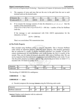
c) The minimum hamming distance = _____________.
d) The no. of errors this code can detect is ____________
e) The no. of errors this code can correct is ____________
f) The code rate = ___________________.
g) Is this code a systematic code? Justify your answer. (HINT: see the tabulated code words
obtained in Q1: b)
________________________________________________________________________________
________________________________________________________________________________
________________________________________________________________________________
________________________________________________________________________________
_______________________________________________________
2) Consider a systematic (6, 3) block code generated by the submatrix [1 1 0; 0 1 1; 1 0 1].
a) Write the value of n and k.
________________________________________________________________________________
________________________________________________________________________________

60. Digital Communication Systems Lab Session 9
NED University of Engineering & Technology – Department of Computer & Information Systems Engineering
57
b) Tabulate the code words through simulation and write their corresponding weights.
MESSAGE CODE VECTOR WEIGHT
000
001
010
011
100
101
110
111
c) What is the value of dmin ?
________________________________________________________________________
3) Write MATLAB code to create 10 messages randomly having size of 4 bits each. Design
appropriate encoding rule and use encode function to encode the generated messages.
________________________________________________________________________________
________________________________________________________________________________
________________________________________________________________________________
________________________________________________________________________________
________________________________________________________________________________
________________________________________________________________________________
4)A digital communication link carries binary coded words representing samples of the following
signal.
X (t) = 300 cos600πt + 2 cos1800πt
The link operates at 1000 samples/sec.
a) Determine the Nyquist rate?
_______________________________________________________________________________________
________________________________________________________________________________

61. Digital Communication Systems Lab Session 9
NED University of Engineering & Technology – Department of Computer & Information Systems Engineering
58
b) Sample the signal using a sampling rate of 1000 samples/sec & determine the DT signal so
obtained.
_______________________________________________________________________________________
________________________________________________________________________________
c) Reconstruct the signal using the sampling rate of 1000 samples/sec
_______________________________________________________________________________________
________________________________________________________________________________
d) Was the original CT signal reconstructed?
_______________________________________________________________________________________
________________________________________________________________________________
e) Perform the above conversion (from CT to DT and extract CT back from the derived DT
signal) using Matlab commands.
_______________________________________________________________________________________
________________________________________________________________________________
_______________________________________________________________________________________
________________________________________________________________________________

62. Digital Communication Systems Lab Session 10
NED University of Engineering & Technology – Department of Computer & Information Systems Engineering
59
Lab Session 10
OBJECT
Decoding linear block codes
THEORY:
Let Y stands for the received vector when a particular code vector X has been transmitted. Any
transmission errors will result in Y ≠ X. The decoder detects or corrects errors in Y using stored
information about the code.
A direct way of performing error detection would be to compare Y with every vector in the code.
This method requires storing all 2k
code vectors at the receiver and performing up to 2k
comparisons. But efficient codes generally have large values of k, which implies rather extensive
and expensive decoding hardware.
More practical decoding methods for codes with large k involve parity check information derived
from the code’s P submatrix. Associated with any systematic linear (n,k) block code is a (n-k)
× n matrix called the parity check matrix H. This matrix is defined by
H = [P’ | Ir]
Where Ir is the r × r identity matrix and n - k = r. The parity check matrix has a crucial
property for error detection which is
XHT
= (0 0 0 0 ……..0)
provided that X belongs to the set of code vectors. However, when Y is not a code vector, the
product YHT
contains at least one nonzero element.
Therefore, given HT
and a received vector Y, error detection can be based on
S = Y HT
an r-bit vector called the syndrome. If all elements of S equal zero, then either Y equals the
transmitted vector X and there are no transmission errors, or Y equals some other code vector and
the transmission errors are undetectable. Otherwise, errors are indicated by the presence of nonzero
elements in S. Thus a decoder for error detection simply takes the form of a syndrome calculator.
We develop the decoding method by introducing an n-bit error vector E whose non zero elements
mark the positions of transmission errors in Y. For instance, if X = (1 0 1 1 0) and Y = (1 0 0 1 1)
then E = (0 0 1 0 1). In general,
Y = X  E
And conversely,
X = Y  E
Substituting Y = X + E into S = YHT
, we obtain
S = (X E)HT
S =XHT
 EHT

63. Digital Communication Systems Lab Session 10
NED University of Engineering & Technology – Department of Computer & Information Systems Engineering
60
S = EHT
which reveals that the syndrome depends entirely on the error pattern, not the specific transmitted
vector.
Syndrome decoding: example
An (8, 4) binary linear block code C is defined by systematic matrices:
1 0 0 0 | 0 1 1 1 0 1 1 1 | 1 0 0 0
G = 0 1 0 0 | 1 0 1 1 H = 1 0 1 1 | 0 1 0 0
0 0 1 0 | 1 1 0 1 1 1 0 1 | 0 0 1 0
0 0 0 1 | 1 1 1 0 1 1 1 0 | 0 0 0 1
Consider two possible messages:
m1 = [0 1 1 0] m2 = [1 0 1 1]
c1 = [0 1 1 0 0 1 1 0] c2 = [0 1 0 0 1 0 1 1]
Suppose error pattern e = [0 0 0 0 0 1 0 0] is added to both code words.
r1 = [0 1 1 0 0 0 1 0] r2 = [0 1 0 0 1 1 1 1]
Calculating the syndrome using S = YHT
. Here Y is the received erroneous code word.
s1 = [0 1 0 0] s2 = [0 1 0 0]
The syndromes are the same and equal column 6 of H, so decoder corrects bit 6.
Bit Error Rate:
Bit error rate = average no. of erroneous bits per block / total no. of bits per block
MATLAB FUNCTIONS:
In order to develop MATLAB code for decoding and calculating the bit error rate, the following
functions may be used.
1) DECODE:
Function: Block decoder
Syntax
msg = decode(code,n,k,'linear/fmt',genmat,trt)
[msg,err] = decode(...)
[msg,err,ccode] = decode(...)
[msg,err,ccode,cerr] = decode(...)
trt Uses syndtable to create the syndrome decoding table associated with the method's
parity-check matrix. Syndtable function is described later in this lab session.
Description
The decode function aims to recover messages that were encoded using an error-correction coding
technique. The technique and the defining parameters must match those that were used to encode
the original signal.
Lab session #2 explains the meanings of n and k, the possible values of fmt, and the possible
formats for msg and code for the encode function. You should be familiar with the conventions

64. Digital Communication Systems Lab Session 10
NED University of Engineering & Technology – Department of Computer & Information Systems Engineering
61
described there. Using the decode function with an input argument code that was not created by
the encode function might cause errors.
Decode function decodes code, which is a linear block code determined by the k-by-n generator
matrix genmat. genmat is required as input. decode tries to correct errors using the decoding
table trt, where trt is a 2^(n-k)-by-n matrix.
[msg,err] = decode(...) returns a column vector err that gives information about error
correction. A nonnegative integer in the rth row of err (or the rth
row of vec2mat(err,k) if
code is a column vector) indicates the number of errors corrected in the rth
message word. A
negative integer indicates that there are more errors in the rth
word than can be corrected.
[msg,err,ccode] = decode(...) returns the corrected code in ccode.
[msg,err,ccode,cerr] = decode(...) returns a column vector cerr whose meaning
depends on the format of code:
 If code is a binary vector, then a nonnegative integer in the rth
row of vec2mat(cerr,n)
indicates the number of errors corrected in the rth
codeword. A a negative integer indicates
that there are more errors in the rth
codeword than can be corrected.
 If code is not a binary vector, then cerr = err.
2) SYNDTABLE:
Function: Produces syndrome decoding table
Syntax:
t = syndtable(h)
Description
t = syndtable(h) returns a decoding table for an error-correcting binary code having codeword
length n and message length k. h is an (n-k)-by-n parity-check matrix for the code. t is a 2n-k
-
by-n binary matrix. The rth
row of t is an error pattern for a received binary codeword whose
syndrome has decimal integer value r-1. (The syndrome of a received codeword is its product with
the transpose of the parity-check matrix.).
3) BITERR:
Function: Computes number of bit errors and bit error rate.
Syntax
[number,ratio] = biterr(x,y)

65. Digital Communication Systems Lab Session 10
NED University of Engineering & Technology – Department of Computer & Information Systems Engineering
62
Description
The biterr function compares unsigned binary representations of elements in vector x with those in
vector y.
Each element of x and y must be a nonnegative decimal integer; biterr converts each element
into its natural unsigned binary representation. number is a scalar or vector that indicates the
number of bits that differ. ratio is number divided by the total number of bits. The total number
of bits, the size of number, and the elements that biterr compares are determined by the
dimensions of x and y.
Biterr function compares the elements in x and y. If the largest among all elements of x and y
has exactly k bits in its simplest binary representation, then the total number of bits is k times the
number of entries in the smaller input. The sizes of x and y determine which elements are
compared:
 If x and y are matrices of the same dimensions, then biterr compares x and y element by
element. number is a scalar. See the figure given below.
If one is a row (respectively, column) vector and the other is a two-dimensional matrix, then biterr
compares the vector element by element with each row (resp., column) of the matrix. The length of
the vector must equal the number of columns (resp., rows) in the matrix. number is a column (resp.,
row) vector whose mth entry indicates the number of bits that differ when comparing the vector
with the mth row (resp., column) of the matrix. See schematics in the given figures.
4) gen2par
Function: Convert between parity-check and generator matrices
Syntax
parmat = gen2par(genmat)
genmat = gen2par(parmat)
X1
X2
X3
X4
X5
X6
Y1
Y2
Y3
Y4
Y5
Y6
Y
XYX

66. Digital Communication Systems Lab Session 10
NED University of Engineering & Technology – Department of Computer & Information Systems Engineering
63
Description
parmat = gen2par(genmat) converts the standard-form binary generator matrix genmat into
the corresponding parity-check matrix parmat.
genmat = gen2par(parmat) converts the standard-form binary parity-check matrix parmat
into the corresponding generator matrix genmat.
The standard forms of the generator and parity-check matrices for an [n,k] binary linear block
code are shown in the table below.
Type of Matrix Standard Form Dimensions
Generator [Ik | P] or [P | Ik] k-by-n
Parity-check [P' | In-k] or [In-k | P'] (n-k)-by-n
where Ik is the identity matrix of size k and the ' symbol indicates matrix transpose. Two standard
forms are listed for each type, because different authors use different conventions.
Example 1
The command below compares the column vector [0; 0; 0] to each column of a random binary
matrix. The output is the number and proportion of 1s in the matrix.
[number,ratio] = biterr([0;0;0],randint(3,5))
The output is
number =
2 1 1 0 1
ratio =
0.6667 0.3333 0.3333 0 0.3333
Example 2
The script below adds errors to 10% of the elements in a matrix. Each entry in the matrix is a two-
bit number in decimal form. The script computes the bit error rate using biterr.
x = randint(100,100,4); % Original signal
% Create errors to add to ten percent of the elements of x.
% Errors can be either 1, 2, or 3 (not zero).
errorplace = (rand(100,100) > .9); % Where to put errors
errorvalue = randint(100,100,[1,3]); % Value of the errors

67. Digital Communication Systems Lab Session 10
NED University of Engineering & Technology – Department of Computer & Information Systems Engineering
64
errors = errorplace.*errorvalue;
y = rem(x+errors,4); % Signal with errors added, mod 4
[num_bit,ratio_bit] = biterr(x,y,2)
The output is
num_bit = 1304
ratio_bit = 0.0652
Example 3
The commands below convert the parity-check matrix for a Hamming code into the corresponding
generator matrix and back again.
parmat = hammgen(3)
genmat = gen2par(parmat)
parmat2 = gen2par(genmat) % Ans should be the same as parmat above
The output is
parmat =
1 0 0 1 0 1 1
0 1 0 1 1 1 0
0 0 1 0 1 1 1
genmat =
1 1 0 1 0 0 0
0 1 1 0 1 0 0
1 1 1 0 0 1 0
1 0 1 0 0 0 1
parmat2 =
1 0 0 1 0 1 1
0 1 0 1 1 1 0
0 0 1 0 1 1 1
The above example uses hammgen function whose explanation is as follows.
h = hammgen(m)
The codeword length is n. n has the form 2m
-1 for some positive integer m greater than or equal to
3. The message length, k, has the form n-m. hammgen function produces an m-by-n parity-check
matrix for a Hamming code having codeword length n = 2m-1
. The input m is a positive integer
greater than or equal to 3. The message length of the code is n-m.
You can also provide your own generator matrix as input.

68. Digital Communication Systems Lab Session 10
NED University of Engineering & Technology – Department of Computer & Information Systems Engineering
65
Example 4
The next example creates a linear code, adds noise, and then decodes the noisy code. It uses the
decode function.
n = 3; k = 2; % A (3,2) linear code
msg = randint(100,k,[0,1]); % 100 messages, k bits each
code = encode(msg,n,k,'linear/binary');
% Add noise.
noisycode = rem(code + randerr(100,n,[0 1;.7 .3]), 2);
newmsg = decode(noisycode,n,k,'linear'); % Try to decode.
% Compute error rate for decoding the noisy code.
[number,ratio] = biterr(newmsg,msg);
disp(['The bit error rate is ',num2str(ratio)])
The output is below.
Your error rate results might vary because the noise is random.
The bit error rate is 0.08

69. Digital Communication Systems Lab Session 10
NED University of Engineering & Technology – Department of Computer & Information Systems Engineering
66
EXERCISES
1: Apply table lookup decoding to (7,4) hamming code. The P submatrix is given as
a)Write the value of n and k.
___________________________________________________________________________
b) Create G and H matrices.
________________________________________________________________________________
________________________________________________________________________________
________________________________________________________________________________
________________________________________________________________________________
________________________________________________________________________________
________________________________________________________________________________
________________________________________________________________________________
________________________________________________________________________________
________________________________________________________________________________
c) Tabulate the code words through simulation and write their corresponding weights.
Message Code Vector Weights
0000
0001
0010
0011
0100
0101
0110
1 0 1
1 1 1
1 1 0
0 1 1

70. Digital Communication Systems Lab Session 10
NED University of Engineering & Technology – Department of Computer & Information Systems Engineering
67
0111
1000
1001
1010
1011
1110
1111
d) The minimum hamming distance = _____________.
e) The no. of errors this code can detect is
________________________________________________________________________________
________________________________________________________________________________
f) The no. of errors this code can correct is
________________________________________________________________________________
________________________________________________________________________________
g) Find syndromes for all possible single error patterns.
S E
0 0 0 0 0 0 0 0 0 0
1 0 1 1 0 0 0 0 0 0

71. Digital Communication Systems Lab Session 10
NED University of Engineering & Technology – Department of Computer & Information Systems Engineering
68
h) Suppose a received word happens to have two errors, such that E = (1 0 0 0 0 1 0). Calculate the
syndrome.
________________________________________________________________________________
________________________________________________________________________________
________________________________________________________________________________
________________________________________________________________________________
i) What will be the error pattern (write form table).
________________________________________________________________________________
j) Write the corrected word.
________________________________________________________________________________
k) What observations do you make? How many errors the decoded output word will contain.
________________________________________________________________________________
________________________________________________________________________________
________________________________________________________________________________
2) Write MATLAB code to construct lookup table for the (6,3) block code generated by the
submatrix
________________________________________________________________________________
________________________________________________________________________________
________________________________________________________________________________
________________________________________________________________________________
________________________________________________________________________________
________________________________________________________________________________
________________________________________________________________________________
________________________________________________________________________________
________________________________________________________________________________
________________________________________________________________________________
________________________________________________________________________________
1 1 0
0 1 1
1 0 1

72. Digital Communication Systems Lab Session 10
NED University of Engineering & Technology – Department of Computer & Information Systems Engineering
69
________________________________________________________________________________
________________________________________________________________________________
________________________________________________________________________________
________________________________________________________________________________
________________________________________________________________________________
________________________________________________________________________________
3) Consider a (5,3) block code obtained by deleting the last column of the P submatrix in the
previous question. Construct the lookup table and show that this code could be used for error
detection and not correction. Also write MATLAB code to implement the given functionality.
________________________________________________________________________________
________________________________________________________________________________
________________________________________________________________________________
________________________________________________________________________________
________________________________________________________________________________
________________________________________________________________________________
________________________________________________________________________________
________________________________________________________________________________
________________________________________________________________________________
________________________________________________________________________________
________________________________________________________________________________
________________________________________________________________________________
________________________________________________________________________________
________________________________________________________________________________
________________________________________________________________________________
________________________________________________________________________________
________________________________________________________________________________
________________________________________________________________________________
________________________________________________________________________________
________________________________________________________________________________
________________________________________________________________________________
________________________________________________________________________________
________________________________________________________________________________

73. Digital Communication Systems Lab Session 10
NED University of Engineering & Technology – Department of Computer & Information Systems Engineering
70
________________________________________________________________________________
________________________________________________________________________________
________________________________________________________________________________
4) A (7,4) LBC has generator matrix G given by
a) Determine the PCM for above matrix.
________________________________________________________________________________
________________________________________________________________________________
________________________________________________________________________________
________________________________________________________________________________
________________________________________________________________________________
b) Write MATLAB code to encode all possible data words and then decode all the encoded words.
________________________________________________________________________________
________________________________________________________________________________
________________________________________________________________________________
________________________________________________________________________________
________________________________________________________________________________
________________________________________________________________________________
________________________________________________________________________________
________________________________________________________________________________
________________________________________________________________________________
________________________________________________________________________________
________________________________________________________________________________
________________________________________________________________________________
________________________________________________________________________________
________________________________________________________________________________
________________________________________________________________________________
1 0 0 0 1 1 0
0 1 0 0 1 0 1
0 0 1 0 0 1 1
0 0 0 1 1 1 1

74. Digital Communication Systems Lab Session 10
NED University of Engineering & Technology – Department of Computer & Information Systems Engineering
71
________________________________________________________________________________
________________________________________________________________________________
c) Insert double error in any code block. Decode manually and through simulation.
________________________________________________________________________________
________________________________________________________________________________
________________________________________________________________________________
________________________________________________________________________________
________________________________________________________________________________
________________________________________________________________________________
________________________________________________________________________________
________________________________________________________________________________
________________________________________________________________________________
d) The bit error rate for single error in first two code blocks is
________________________________________________________________________________
________________________________________________________________________________
________________________________________________________________________________
________________________________________________________________________________
e) Insert single error in every code block. Write MATLAB code to find bit error rate.
________________________________________________________________________________
________________________________________________________________________________
________________________________________________________________________________
________________________________________________________________________________
________________________________________________________________________________
________________________________________________________________________________
________________________________________________________________________________

75. Digital Communication Systems Lab Session11
NED University of Engineering & Technology – Department of Computer & Information Systems Engineering
72
Lab Session 11
OBJECT
Introduction to Cyclic codes.
THEORY
Cyclic codes are a subclass of linear block codes with a cyclic structure that leads to more
practical implementation. Block codes used in forward error correction systems are almost
always cyclic codes.
In cyclic coding, data is sent with a checksum. When arrives, checksum is recalculated. It
should match the one that was sent.
To describe a cyclic code, we express an arbitrary n-bit vector in the form
X = (xn-1 xn-2 ……………x1 x0)
Now suppose that X has been loaded into a shift register with feedback connection from the
first to last stage. Shifting all bits one position to the left yields the cyclic shift of X, written as
X'
= (xn-2 xn-3 ……………x1 x0 xn-1)
A second shift produces
X’’
= (xn-3 ……………x1 x0 xn-1 xn-2) and so forth.
A linear code is cyclic if every cyclic shift of a code vector X is another vector in the code.
Since cyclic codes are linear block codes, all the properties of linear block codes apply to
cyclic codes.
Cyclic codes are used in applications where burst errors can occur. Burst error is an error in
which a group of adjacent bits is affected.
Encoding of Cyclic Codes
Direct Approach:
Let M(x) is the message polynomial and G(x) is the generator polynomial. Then the code
vector V(x) can be encoded as
V(x) = M(x). G(x)
A linear code is cyclic if every cyclic shift of a code vector X is another vector in the code.
Example 1
The (6, 2) repetition code having valid code C = {[000000], [010101], [101010], [111111]} is
cyclic, since a cyclic shift of any of its code vectors results in a vector that is an element of C.

76. Digital Communication Systems Lab Session11
NED University of Engineering & Technology – Department of Computer & Information Systems Engineering
73
Example 2
The (5, 2) LBC is defined by the generator matrix G = [1 0 1 1 1; 0 1 1 0 1] is a single error
correcting code. We need to determine if it is cyclic.
The valid code words are
C = {[00000], [01101], [10111], [11010]}
The given code is NOT a cyclic code because cyclic shift of (11010) results in (10101) which
is not a valid code word. Also cyclic shift of (10111) results in (01111) which is not a member
of C.
It is convenient to think of words as polynomials rather than vectors. Since the code is binary,
the coefficients will be 0 or 1. The degree of polynomial equals to its highest exponent. For
example the degree of the polynomial obtained from (1 0 1 1) is 3
Example 3
Express (1101) as polynomial. We always write most significant digit on the left.
(1101) can be expressed as 1.x3
+ 1.x2
+ 0.x1
+ 1.x0
or x3
+ x2
+ 1
Special case: We don't allow bit string = all zeros.
110001 represents:
1.x5
+ .x4
+ 0.x3
+ 0.x2
+ 0.x1
+ 1.x0
= x5
+ x4
+ x0
The order of a polynomial is the power of the highest non-zero coefficient. This is polynomial
of order 5.
A cyclic code with the generator polynomial of degree (n-k) detects all burst errors affecting
n-k bits or less.
Where
n = number of bits in code word.
k = number of bits in data word.
Encoding involves multiplying data Polynomial (message polynomial) by generator
polynomial.
V(x) = M(x). G(x)
Calculations are performed as
Multiplication modulo2 = AND
Addition modulo2 = XOR

77. Digital Communication Systems Lab Session11
NED University of Engineering & Technology – Department of Computer & Information Systems Engineering
74
Example 4
Given (6, 3) code with G(x) = (1 1 0 1). Encode M(x) = (101)
V(x) = M(x). G(x)
V(x) = (x3
+ x2
+ 1). (x2
+ 1)
V(x) = x5
+ x3
+ x4
+ x2
+ x2
+ 1
V(x) = 1.x5
+ 1.x4
+ 1.x3
+ (1  1) x2
+ 0.x + 1
V(x) = 1.x5
+ 1.x4
+ 1.x3
+ 0.x2
+ 0.x + 1
V(x) = (1 1 1 0 0 1)
The degree of polynomial is defined to be the highest power of x in the polynomial for which
the coefficient of x is not zero. The degree of polynomial M(x) is denoted by deg [M(x)].
If M is our set of k bit source vectors, the highest degree polynomial in the set of polynomials
M(x) that describes our source vectors is k-1. If deg [G(x)] = r, then the highest degree
of our set of code polynomials V(x) is n-1 or k-1+r. Therefore deg [G(x)] tells us the
number of check bits in the code.
Property of generator Polynomial
G(x) is the generator polynomial for a linear cyclic code of length n if and only if G(x)
divides 1+xn
without a remainder.
Example 5
Given (7, 4) cyclic code. Find a generator polynomial for a code of length n = 7 for encoding
of data of length k = 4.
Solution:
G(x) should be a degree 7 – 4 = 3 and should divide 1 + xn
without a remainder.
1 + x7
can be factorized as
1 + x7
= (1+x+x3
) (1+x2
+x3
) (1+x)
So we can choose for G(x) either (1+x+x3
) or (1+x2
+x3
).
Systematic form:
Let
U(x) = uk-1 xk-1
+ uk-2 xk-2
+ ... + u1 x+ u0 be an information polynomial and
G (x) = g n - k x n - k
+ g n - k - 1xn -k-1
+... + g1 x + g0 be a generator polynomial of an (n, k) cyclic
code. The code polynomial is given by
V(x) = xn-k
U(x) / G(x)
= Vs(x) / G(x)
Where
Vs(x) = x n -k
U(x)

78. Digital Communication Systems Lab Session11
NED University of Engineering & Technology – Department of Computer & Information Systems Engineering
75
Systematic encoding of an (n, k) cyclic code consists of multiplying U(x) by xn-k
, then
computing the remainder b(x) of xn-k
U(x) / G(x), and forming the code polynomial
V(x). A linear (n - k)-stage shift register with feedback connections circuit can
simultaneously accomplish the multiplication and division tasks.
This systematic encoding form a class of cyclic codes called “Cyclic Redundancy Check”.
Cyclic Redundancy check or CRC codes are error detecting codes typically used in automatic
repeat request systems. CRC codes have no error correction capability but they can be used in
combination with an error correcting code. When used in this fashion, the error control system
is in the form of a concatenated code. CRC codes are generated and their syndromes are
calculated in precisely the same manner as other cyclic codes. Since these codes are error
detecting rather than error correcting, there is no error correction circuit. Instead, the
syndrome of the received block is checked to see if it is ZERO (no error detected) or NON
ZERO (error detected).
Example 6
Consider a message 110010 represented by the polynomial
M(x) = x5
+ x4
+ x
Consider a generating polynomial
G(x) = x3
+ x2
+ 1 (1101)
This is used to generate a 3 bit CRC = C(x) to be appended to M(x).
STEPS:
1. Multiply M(x) by x3
(highest power in G(x)). I.e. Add 3 zeros. 110010000
2. Divide the result by G(x). The remainder = C(x). 1101 long division into 110010000
(with subtraction mod 2) = 100100 remainder 100
Special case: This won't work if bit string = all zeros. We don't allow such an
M(x).
Transmit 110010000 + 100. To be precise, transmit: T(x) = x3
M(x) + C(x)
= 110010100
3. Receiver end: Receive T(x). Divide by G(x), should have remainder 0.
Example 7
The following example shows the long division of message word (1101011011) by the
generator (10011)
The remainder obtained is appended (added) to the frame to form the transmitted vector.
Highest power of generator polynomial is ‘4’

79. Digital Communication Systems Lab Session11
NED University of Engineering & Technology – Department of Computer & Information Systems Engineering
76
Receiver end: Receive T(x). Divide by G(x), should have remainder 0; verify it yourself.

80. Digital Communication Systems Lab Session11
NED University of Engineering & Technology – Department of Computer & Information Systems Engineering
77
DECODING
Let T(x) and E(x) be the code polynomial of a systematic cyclic code and an error polynomial
of degree n - 1 or less, respectively. An error is the same as adding some E(x) to T(x) for
e.g. adding 1010011000001110000 will flip the bits at the locations where "1" is in the error
bit string. Instead of T(x) arriving, T(x)  + E(x) arrives.
So R(x) = T(x)  E(x)
In general, each 1 bit in E(x) corresponds to a bit that has been flipped in the message.
If there are k 1 bits in E(x), k single-bit errors have occurred. A burst error looks like 1....1
Far end receives T(x) + E(x) = R(x). T(x) is multiple of G(x) (remainder zero). Hence
remainder when you divide (T(x)  + E(x)) by G(x) = remainder when you divide E(x) by
G(x). For e.g. remainder when divide (1000+n) by 10 = remainder when you divide n by 10
Here the remainder of E(x) / G(x) is called syndrome vector denoted by S(x). If remainder
when you divide E(x) by G(x) is zero, the error will not be detected.
In general, if E(x) is a multiple of G(x), the error will not be detected.
Otherwise, it will. All other error patterns will be caught.
MATLAB FUNCTIONS
1) Encode
Function: Block encoder
Syntax
Code = encode (msg,n,k,'cyclic/fmt',genpoly)
Description
Encode function encodes msg and creates a systematic cyclic code. genpoly is a row vector
that gives the coefficients, in order of ascending powers, of the binary generator polynomial.
The default value of genpoly is cyclpoly (n,k). This function is explained below. By
definition, the generator polynomial for an [n, k] cyclic code must have degree n-k and must
divide xn
-1. You are already familiar with the input arguments ‘msg’, ‘n’ and ‘k’.
2) Cyclpoly
Function: Produce generator polynomials for a cyclic code.
Syntax
pol = cyclpoly (n, k)

81. Digital Communication Systems Lab Session11
NED University of Engineering & Technology – Department of Computer & Information Systems Engineering
78
Description
In MATLAB a polynomial is represented as a row containing the coefficients in order of
ascending powers. The results you would get will be in ascending order of coefficients while
in manual calculation the results will be in descending order. It does not matter what
convention you follow but it should be consistent. Cyclpoly function returns the row vector
representing one nontrivial generator polynomial for a cyclic code having codeword length n
and message length k.
3) Decode
Function: Block decoder
Syntax
msg = decode (code, n ,k, 'cyclic/fmt', genpoly, trt)
[msg, err] = decode (...)
[msg, err, ccode] = decode (...)
[msg, err, ccode, cerr] = decode (...)
Description
decode function decodes the cyclic code ‘code’ and tries to correct errors using the decoding
table ‘trt’, where trt is a 2^(n-k)-by-n matrix. ‘genpoly’ is a row vector that gives the
coefficients, in order of ascending powers, of the binary generator polynomial of the code.
The default value of genpoly is cyclpoly (n, k). By definition, the generator
polynomial for an [n, k] cyclic code must have degree n-k and must divide xn
-1.
‘trt’ uses syndtable to create the syndrome decoding table associated with the method's
parity-check matrix. Syndtable function is explained in lab session 4. The return parameters
‘err’, ‘ccode’ and ‘cerr’ have the same purpose as explained in lab session 4.
Example 8
The following example creates a cyclic code, adds noise, and then decodes the noisy code. It
uses the decode function.
n = 3; k = 2; % A (3, 2) cyclic code
msg = randint(100,k,[0,1]); % 100 messages, k bits each
Code = encode (msg, n, k, 'cyclic/binary'); % Add noise.
noisycode = rem(code + randerr (100,n,[0 1;.7 .3]), 2);
newmsg = decode(noisycode, n, k, 'cyclic'); % Try to decode.
% Compute error rate for decoding the noisy code.
[Number, ratio] = biterr (newmsg, msg);
disp (['The bit error rate is ',num2str(ratio)])

82. Digital Communication Systems Lab Session11
NED University of Engineering & Technology – Department of Computer & Information Systems Engineering
79
Example 9
The example below illustrates the use of ‘err’ and ‘cerr’. The script encodes a five-bit
message using a cyclic code. The codeword has fifteen bits. No Error is added to the
codeword. Then decode is used to recover the original message.
m = 4
n = 2^m-1 % Codeword length is 15.
k = 5 % Message length
msg = ones(1,5) % One message of five bits.
Code = encode (msg,n,k,'cyclic') % Encode the message.
noisycode = code % No error
% decodes and tries to correct the errors.
[newmsg,err,ccode,cerr] = decode (noisycode,n,k,'cyclic')
disp ('Transpose of err is')
disp (err')
disp ('Transpose of cerr is')
disp (cerr')
The Galois Field Computation in MATLAB
A Galois field is an algebraic field that has a finite number of members. Galois fields having
2^m members are used in error-control coding and are denoted GF (2^m) where m is an
integer between 1 and 16. This portion describes how to work with fields that have 2^m
members with m = 0.
4) gf
Function: Creates a Galois field array.
Syntax
x_gf = gf(x,m)
x_gf = gf(x)
Description
x_gf = gf(x,m) creates a Galois field array from the matrix x. The Galois field has 2^m
elements, where m is an integer between 1 and 16. The elements of x must be integers between
0 and 2^m-1. The output x_gf is a variable that MATLAB recognizes as a Galois field array,
rather than an array of integers. As a result, when you manipulate x_gf using operators or
functions such as + or det, MATLAB works within the Galois field you have specified.
X_gf = gf(x) creates a GF (2) array from the matrix x. Each element of x must be 0 or 1.

83. Digital Communication Systems Lab Session11
NED University of Engineering & Technology – Department of Computer & Information Systems Engineering
80
Example 10:
Let
g = [0 1 1; 1 0 1; 1 1 0]
d = [0 1 0]
Run the following statement
c = d*g
Output:
c = 1 0 1
Using d = [1 0 1] rerun the above statement.
Output:
c = 1 2 1
When you perform modulo 2 multiplications on two binary vectors, you get a binary vector as
result. This is not the case here because MATLAB considers these vector elements as
integers. For this purpose we convert the vectors into Galois field of order 2.
Now convert all the given vectors and g matrix to Galois field and do the computation again.
G=gf (g)
D=gf (d)
c=D*G
Array elements =
1 0 1
5) conv
Function: Convolution and polynomial multiplication
Syntax:
w = conv (u,v)
Description:
conv function convolves vectors u and v. Algebraically, convolution is the same operation as
multiplying the polynomials whose coefficients are the elements of u and v.
Example 11:
m = [1 1 0 0 1 0]
g = [1 1 0 1]
Compute c = m*g manually.
Answer: 101101010.
Run the following statement.
c = m*g
Note the error you get.
Convert m and g in to Galois field arrays.

84. Digital Communication Systems Lab Session11
NED University of Engineering & Technology – Department of Computer & Information Systems Engineering
81
M = gf(m)
G = gf(g)
Rerun the statement C=M*G
Now note the error that you get. Despite of the fact that we have converted m and g into
Galois field, still multiplication is not possible because sizes of m and g don’t match.
Now use conv function
C = conv (M, G)
Note that now you get the correct result.
6) deconv
Function: Deconvolution and polynomial division.
Syntax:
[q,r] = deconv (v,u)
Description:
Deconv function deconvolves vector u out of vector v, using long division.
The quotient is returned in vector q and the remainder in vector r such that
v = conv (u,q)+r.
If u and v are vectors of polynomial coefficients, convolving them is equivalent to
multiplying the two polynomials, and deconvolution is polynomial division.
The result of dividing v by u is quotient q and remainder r.
Example 12:
m=[1 1 0 0 1 0]
g=[1 1 0 1]
Using long division we compute (x3
* m) / g manually.
Answer:
Quotient: 100100
Remainder:100
Now perform the same functionality using MATLAB.
M=gf(m)
G=gf(g)
h=[1 0 0 0] % or x3
that is highest power of g(x)
H=gf(h)
C=conv(H,M) % multiplying x3 * m(x)
[q,r]=deconv(C,G) % dividing [x3*m(x)] by g(x)
See that the results you get in both the cases match.

85. Digital Communication Systems Lab Session11
NED University of Engineering & Technology – Department of Computer & Information Systems Engineering
82
EXERCISES
1. The generator polynomial of a (7, 4) cyclic code is given by
G(x) = 1 + x + x3
Find V by direct method as well as the systematic approach if M(x) = (1 0 1 0).
Write code to implement the above functionality in MATLAB using encode function and
then conv function.
___________________________________________________________________________
___________________________________________________________________________
___________________________________________________________________________
___________________________________________________________________________
___________________________________________________________________________
___________________________________________________________________________
___________________________________________________________________________
___________________________________________________________________________
___________________________________________________________________________
___________________________________________________________________________
___________________________________________________________________________
___________________________________________________________________________
___________________________________________________________________________
___________________________________________________________________________
___________________________________________________________________________
___________________________________________________________________________
___________________________________________________________________________
___________________________________________________________________________
___________________________________________________________________________
___________________________________________________________________________
___________________________________________________________________________
___________________________________________________________________________
___________________________________________________________________________
___________________________________________________________________________

86. Digital Communication Systems Lab Session11
NED University of Engineering & Technology – Department of Computer & Information Systems Engineering
83
2. Consider the cyclic (7, 4) cyclic code generated by G(x) = x3
+ x + 1.
a) Use long division to calculate the check bit polynomial C(x) when M = (1 1 0 0). Also
write the complete code polynomial.
___________________________________________________________________________
___________________________________________________________________________
___________________________________________________________________________
___________________________________________________________________________
___________________________________________________________________________
___________________________________________________________________________
___________________________________________________________________________
___________________________________________________________________________
___________________________________________________________________________
___________________________________________________________________________
___________________________________________________________________________
___________________________________________________________________________
___________________________________________________________________________
___________________________________________________________________________
___________________________________________________________________________
___________________________________________________________________________
___________________________________________________________________________
___________________________________________________________________________
b) Write MATLAB code to perform the above functionality. Use encode/decode functions
and then conv/deconv functions.
___________________________________________________________________________
___________________________________________________________________________
___________________________________________________________________________
___________________________________________________________________________
___________________________________________________________________________
___________________________________________________________________________
___________________________________________________________________________
___________________________________________________________________________
___________________________________________________________________________

87. Digital Communication Systems Lab Session11
NED University of Engineering & Technology – Department of Computer & Information Systems Engineering
84
___________________________________________________________________________
___________________________________________________________________________
___________________________________________________________________________
___________________________________________________________________________
___________________________________________________________________________
___________________________________________________________________________
___________________________________________________________________________
___________________________________________________________________________
___________________________________________________________________________
___________________________________________________________________________
___________________________________________________________________________
___________________________________________________________________________
3. The generator polynomial of (7, 4) cyclic codes is given by G(x) = 1 + x2
+ x3
. Find V by
the systematic approach if M(x) = (1 0 0 1).Let the received word is [1 1 1 0 0 1 1]. Find the
syndrome vector.
___________________________________________________________________________
___________________________________________________________________________
___________________________________________________________________________
___________________________________________________________________________
___________________________________________________________________________
___________________________________________________________________________
___________________________________________________________________________
___________________________________________________________________________
___________________________________________________________________________
___________________________________________________________________________
___________________________________________________________________________
___________________________________________________________________________
___________________________________________________________________________
___________________________________________________________________________
___________________________________________________________________________
___________________________________________________________________________
___________________________________________________________________________
___________________________________________________________________________

88. Digital Communication Systems Lab Session11
NED University of Engineering & Technology – Department of Computer & Information Systems Engineering
85
4. Consider the cyclic (7, 4) hamming code generated by G(x) = x3
+ x + 1.
a) Use systematic approach to calculate the check bit polynomial C(x) when M = (1 1 0 1).
Also write the complete code polynomial.
___________________________________________________________________________
___________________________________________________________________________
___________________________________________________________________________
___________________________________________________________________________
___________________________________________________________________________
___________________________________________________________________________
___________________________________________________________________________
___________________________________________________________________________
___________________________________________________________________________
___________________________________________________________________________
___________________________________________________________________________
___________________________________________________________________________
___________________________________________________________________________
___________________________________________________________________________
___________________________________________________________________________
___________________________________________________________________________
___________________________________________________________________________
___________________________________________________________________________
b) Write MATLAB code to implement the functionality explained in part (a).
___________________________________________________________________________
___________________________________________________________________________
___________________________________________________________________________
___________________________________________________________________________
___________________________________________________________________________
___________________________________________________________________________
___________________________________________________________________________
___________________________________________________________________________
___________________________________________________________________________
___________________________________________________________________________

89. Digital Communication Systems Lab Session11
NED University of Engineering & Technology – Department of Computer & Information Systems Engineering
86
c) Find the syndrome vectors for the following erroneous received words.
i. 1010101
ii. 1000001
iii. 1011001
iv. 1010000
v. 1010011
___________________________________________________________________________
___________________________________________________________________________
___________________________________________________________________________
___________________________________________________________________________
___________________________________________________________________________
___________________________________________________________________________
___________________________________________________________________________
___________________________________________________________________________
___________________________________________________________________________
___________________________________________________________________________
___________________________________________________________________________
___________________________________________________________________________
___________________________________________________________________________
___________________________________________________________________________
___________________________________________________________________________
___________________________________________________________________________
___________________________________________________________________________
___________________________________________________________________________
___________________________________________________________________________
___________________________________________________________________________
___________________________________________________________________________
___________________________________________________________________________
___________________________________________________________________________
___________________________________________________________________________
___________________________________________________________________________
___________________________________________________________________________
___________________________________________________________________________

90. Digital Communication Systems Lab Session11
NED University of Engineering & Technology – Department of Computer & Information Systems Engineering
87
___________________________________________________________________________
___________________________________________________________________________
___________________________________________________________________________
___________________________________________________________________________
___________________________________________________________________________
___________________________________________________________________________
___________________________________________________________________________
___________________________________________________________________________
___________________________________________________________________________
___________________________________________________________________________
___________________________________________________________________________
5) Consider (6, 3) cyclic code. Create MATLAB code to perform the following tasks.
a) Create generator polynomial.
___________________________________________________________________________
___________________________________________________________________________
___________________________________________________________________________
___________________________________________________________________________
b) Write all possible code words and encode using ‘encode’ function.
___________________________________________________________________________
___________________________________________________________________________
___________________________________________________________________________
___________________________________________________________________________
___________________________________________________________________________
___________________________________________________________________________
___________________________________________________________________________
___________________________________________________________________________
c) Use ‘decode’ function to decode all the encoded words.
___________________________________________________________________________
___________________________________________________________________________
___________________________________________________________________________
___________________________________________________________________________

91. Digital Communication Systems Lab Session11
NED University of Engineering & Technology – Department of Computer & Information Systems Engineering
88
d) Induce single error in all the encoded words and then decode. Record the output that you
get.
___________________________________________________________________________
___________________________________________________________________________
___________________________________________________________________________
___________________________________________________________________________
___________________________________________________________________________
___________________________________________________________________________
___________________________________________________________________________
___________________________________________________________________________
___________________________________________________________________________
___________________________________________________________________________

92. Digital Communication Systems Lab Session12
NED University of Engineering & Technology – Department of Computer & Information Systems Engineering
89
Lab Session 12
OBJECT
Understanding loss less data compression using Huffman coding.
THEORY
Huffman coding
Huffman coding is a compression method that converts characters into variable length bit
strings. Most-frequently occurring characters are converted to shortest bit strings; least
frequent, the longest.
In computer science and information theory, Huffman coding is an encoding algorithm used
for lossless data compression. The term refers to the use of a variable-length code table for
encoding a source symbol (such as a character in a file) where the variable-length code table
has been derived in a particular way based on the estimated probability of occurrence for each
possible value of the source symbol. It was developed by David A. Huffman while he was a
Ph.D. student at MIT, and published in the 1952 paper "A Method for the Construction of
Minimum-Redundancy Codes."
Huffman coding uses a specific method for choosing the representation for each symbol,
resulting in a prefix-free code (sometimes called "prefix codes") (that is, the bit string
representing some particular symbol is never a prefix of the bit string representing any other
symbol) that expresses the most common characters using shorter strings of bits than are used
for less common source symbols. Huffman was able to design the most efficient compression
method of this type: no other mapping of individual source symbols to unique strings of bits
will produce a smaller average output size when the actual symbol frequencies agree with
those used to create the code.
BASIC TECHNIQUE
Assume you have a source generating 4 different symbols {a1, a2, a3, a4} with probability
{0.4; 0.35; 0.2; 0.05}. Generate a binary tree from left to right taking the two less probable
symbols, putting them together to form another equivalent symbol having a probability that
equals the sum of the two symbols. Keep on doing it until you have just one symbol. Then
read the tree backwards, from right to left, assigning different bits to different branches as
shown in figure.

93. Digital Communication Systems Lab Session12
NED University of Engineering & Technology – Department of Computer & Information Systems Engineering
90
The final Huffman code is:
Symbol Code
a1 0
a2 10
a3 111
a4 110
The standard way to represent a signal made of 4 symbols is by using 2 bits/symbol, but the
entropy of the source is 1.73 bits/symbol. If this Huffman code is used to represent the signal,
then the entropy is lowered to 1.83 bits/symbol.
Flow Chart of Huffman Algorithm:
Example 1:
Information to be transmitted over the internet contains the following characters with their
associated frequencies:
Character a e l n o s t
Frequency 45 65 13 45 18 22 53
Sort out in ascending
order of probability.
Merge the two least
probable symbols.
No. of
elements
=2
Assign 0 and 1 to
codeword.
If there is
any merger
of two
elements
STOP
Append the
codeword with 0
and 1
No Yes
Yes
No

94. Digital Communication Systems Lab Session12
NED University of Engineering & Technology – Department of Computer & Information Systems Engineering
91
Use Huffman technique to answer the following questions:
a. Build the Huffman code tree for the message.
b. Use the Huffman tree to find the codeword for each character.
c. If the data consists of only these characters, what is the total number of bits to
be transmitted? What is the compression ratio?
d. Verify that your computed Huffman code words satisfy the Prefix property.
Solution:
a)
Step 1: Arrange all characters according to ascending order of frequency as shown in the
following figure
Fig 6.2.1
Step 2: Combine the two least frequently occurring alphabets. Here we combine l (frequency
13) and o (frequency 18) making total of 31. Use the following figure
Fig 6.2.1
Step 3: Now combine 31 with s (frequency 22) forming total 53 as shown in the following
figure.
Fig 6.2.1
13
l
18
0
22
s
45
a
45
n
53
t
65
e
13
l
18
0
22
s
45
a
45
n
53
t
65
e
31
13
l
18
0
22
s
45
a
45
n
53
t
65
e
31
53

95. Digital Communication Systems Lab Session12
NED University of Engineering & Technology – Department of Computer & Information Systems Engineering
92
Step 4: Combining a (frequency 45) and n (frequency 45) making total 90. ‘a’ and ‘n’ are
now least frequent among all as shown in the following figure.
Fig 6.2.1
Step 5: Now combining 53 which was obtained by adding s (22) and 31(l + o) with t
(frequency 53). Here we get total of 106.
Fig 6.2.1
13
l
18
0
22
s 45
a
45
n
53
t
65
e
31
53
90
13
l
18
0
22
s
45
a
45
n
53
t
65
e
31
53
90
106

96. Digital Communication Systems Lab Session12
NED University of Engineering & Technology – Department of Computer & Information Systems Engineering
93
Step 6: Here we add 90 and e (frequency 65) getting 155 as total.
Fig 6.2.1
Step 7: Now we add 155 and 106 and get final sum of 261, as shown.
Fig 6.2.1
13
l
18
0
22
s
45
a
45
n
53
t 65
e
31
53
90
106
155
13
l
18
0
22
s
45
a
45
n
53
t
65
e
31
53
90
106
155
261

97. Digital Communication Systems Lab Session12
NED University of Engineering & Technology – Department of Computer & Information Systems Engineering
94
b) We assign a bit (0 or 1) to every node starting at the leaf and proceeding up the tree (0 =
left, 1 = right).
Fig 6.2.1
The sequence of zeros and ones that are the arcs in the path from the root to each leaf node are
the desired codes:
Character a e l n o s t
Huffman codeword 110 10 0110 111 0111 010 00
c) If we assume the message consists of only the characters a, e, l, n, o, s, t then the number
of bits for the compressed message will be 696:
Character a e l n o s t
Code words 110 10 0110 111 0111 010 00
Code word bits 3 2 4 3 4 3 2
Character frequency 45 65 13 45 18 22 53
Code word bits
frequency
135 130 52 135 72 66 106
SUM = 696
If the message is sent uncompressed with 8-bit ASCII representation for the characters, we
have 261*8 = 2088 bits.
13
l
18
0
22
s
45
a
45
n
53
t
65
e
31
53
90
106
155
2610
1
0 1
1
1
0
0
0

98. Digital Communication Systems Lab Session12
NED University of Engineering & Technology – Department of Computer & Information Systems Engineering
95
ii. The sequence of zeros and ones that are the arcs in the path from the root to each
terminal node are the desired codes:
Character a e l n o s t
Codeword 111 10 0010 110 0011 000 01
iii. If we assume the message consists of only the characters a, e, l, n, o, s, t then the
number of bits transmitted will be:
2*65+2*53+3*45+3*45+3*22+4*18+4*13 = 696 bits + number of bits for Huffman
code tree.
If the message is sent uncompressed with 8-bit ASCII representation for the
characters, we have
261*8 = 2088 bits
That is we saved about 70% transmission time.
d) The Prefix Property
Data encoded using Huffman coding is uniquely decodable. This is because Huffman
codes satisfy an important property called the prefix property. This property guarantees
that no codeword is a prefix of another Huffman codeword. For example, 10 and 101
cannot simultaneously be valid Huffman code words because the first is a prefix of the
second. Thus, any bit stream is uniquely decodable with a given Huffman code. We can
see by inspection that the code words we generated are valid Huffman code words. To see
why the prefix property is essential, consider the code words given below in which “e” is
encoded with 110 which is a prefix of “f”.
character a b c d e f
codeword 0 101 100 111 110 1100
The decoding of 11000100110 is ambiguous:
11000100110 => face
11000100110 => eaace
e) Encode (compress) the message tenseas using the following code words:
Character a e l n o s t
Huffman codeword 110 10 0110 111 0111 010 00
Answer: Replace each character with its codeword:
001011101010110010

99. Digital Communication Systems Lab Session12
NED University of Engineering & Technology – Department of Computer & Information Systems Engineering
96
f) Decode (decompress) each of the following encoded messages, if possible, using the
Huffman codeword tree obtained above
a) 0110011101000
b) 11101110101011
Answer: Decode a bit-stream by starting at the root and proceeding down the tree according
to the bits in the message (0 = left, 1 = right). When a leaf is encountered, output the
character at that leaf and restart at the root .If a leaf cannot be reached, the bit-stream cannot
be decoded.
(a) 0110011101000
0110 corresponds to l, 0111 corresponds to o, 010 is the code for s and 00 is the code for t.
So the given stream is decoded to the word lost.
(b) 11101110101011
Here 111 correspond to n, 0111 corresponds to o, 010 is the code for s.
The decoding fails because the corresponding node for 11 is not a leaf.
Assume that the numbers of character-codeword pairs are included at the beginning of the
binary file containing the compressed message in the format as shown in fig
In binary
(Significant bits).
Characters are in 8-bit
ASCII codes.
Number of bits for the transmitted file = bits (7) + bits (characters) + bits (code words) +
Bits (compressed message)
= 3 + (7*8) +21 + 696
= 776
Compression Ratio = bits for ASCII representation / number of bits transmitted
= 2088 / 776
= 2.69
Thus, the size of the transmitted file is 100 / 2.69 = 37.17 % of the original ASCII file (i.e. 37
% compression has been achieved)
7
a110
e10
l0110
n111
o0111
s010
t00
Sequence of zeroes and ones for the compressed
message.

100. Digital Communication Systems Lab Session12
NED University of Engineering & Technology – Department of Computer & Information Systems Engineering
97
Huffman Coding in MATLAB
In MATLAB Huffman code dictionary associates each data symbol with a codeword. It has
the property that no codeword in the dictionary is a prefix of any other codeword in the
dictionary.
The huffmandict, huffmanenco, and huffmandeco functions support Huffman coding
and decoding.
Creating a Huffman Code Dictionary
dict = huffmandict(symbols, p)
Huffman coding requires statistical information about the source of the data being encoded. In
particular, the p input argument in the huffmandict function lists the probability with which
the source produces each symbol in its alphabet.
For example, consider a data source that produces 1s with probability 0.1, 2s with probability
0.1, and 3s with probability 0.8. The main computational step in encoding data from this
source using a Huffman code is to create a dictionary that associates each data symbol with a
codeword. The commands below create such a dictionary and then show the codeword vector
associated with a particular value from the data source.
symbols = [1 2 3]; % Data symbols
p = [0.1 0.1 0.8]; % Probability of each data symbol
dict = huffmandict(symbols, p) % Create the dictionary.
dict {1,:} % Show first row of the dictionary.
dict {2,:} % Show second row of the dictionary.
dict {3,:} % Show third row of the dictionary.
The output below shows that the most probable data symbol, 3, is associated with a one-digit
codeword, while less probable data symbols are associated with two-digit code words. The
output also shows, for example, that a Huffman encoder receiving the data symbol 1 should
substitute the sequence 11.
dict =
[1] [1x2 double]
[2] [1x2 double]
[3] [ 0]
ans =
1
ans =
1 1

101. Digital Communication Systems Lab Session12
NED University of Engineering & Technology – Department of Computer & Information Systems Engineering
98
ans =
2
ans =
1 0
ans =
3
ans =
0
Creating and Decoding a Huffman Code
The example below performs Huffman encoding and decoding using huffmanenco and
huffmandeco functions. A source is used whose alphabet has three symbols. Notice that the
huffmanenco and huffmandeco functions use the dictionary that huffmandict created.
sig = repmat([3 3 1 3 3 3 3 3 2 3],1,50); % Data to encode
symbols = [1 2 3]; % Distinct data symbols appearing in sig
p = [0.1 0.1 0.8]; % Probability of each data symbol
dict = huffmandict(symbols,p); % Create the dictionary.
hcode = huffmanenco(sig,dict); % Encode the data.
dhsig = huffmandeco(hcode,dict); % Decode the code.
EXERCISES
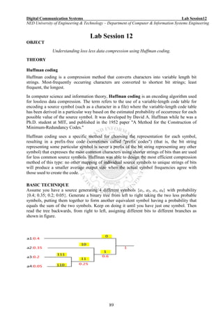
1. Five source symbols of the alphabet of a source and their probabilities are shown
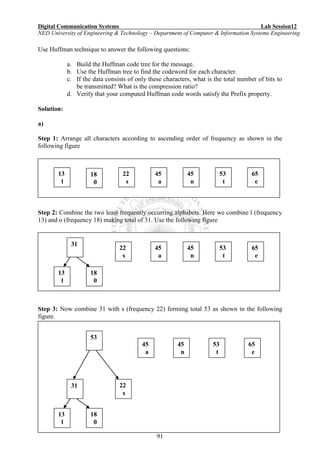
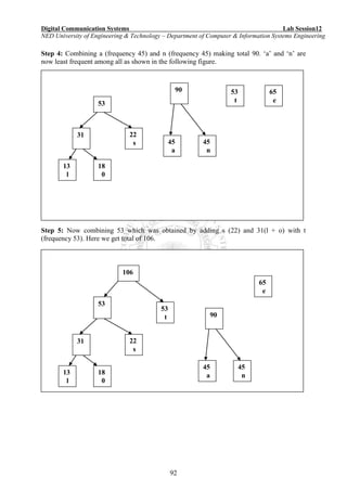
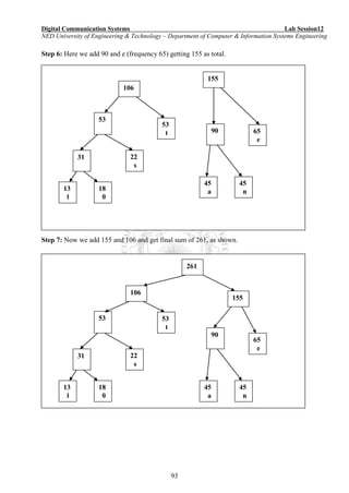
a) Build the Huffman code tree for the message and find the codeword for each character.
___________________________________________________________________________
___________________________________________________________________________
___________________________________________________________________________
___________________________________________________________________________
___________________________________________________________________________
___________________________________________________________________________
Symbol Probability
S0 0.4
S1 0.2
S2 0.2
S3 0.1
S4 0.1

102. Digital Communication Systems Lab Session12
NED University of Engineering & Technology – Department of Computer & Information Systems Engineering
99
___________________________________________________________________________
___________________________________________________________________________
___________________________________________________________________________
___________________________________________________________________________
___________________________________________________________________________
___________________________________________________________________________
___________________________________________________________________________
___________________________________________________________________________
___________________________________________________________________________
___________________________________________________________________________
___________________________________________________________________________
___________________________________________________________________________
___________________________________________________________________________
___________________________________________________________________________
___________________________________________________________________________
___________________________________________________________________________
___________________________________________________________________________
___________________________________________________________________________
b) Write MATLAB code to obtain Huffman coding for the given characters.
___________________________________________________________________________
___________________________________________________________________________
___________________________________________________________________________
___________________________________________________________________________
___________________________________________________________________________
___________________________________________________________________________
___________________________________________________________________________
___________________________________________________________________________
___________________________________________________________________________
___________________________________________________________________________
___________________________________________________________________________
___________________________________________________________________________

103. Digital Communication Systems Lab Session12
NED University of Engineering & Technology – Department of Computer & Information Systems Engineering
100
2. Construct a Huffman code for the source X emitting symbols with probabilities as shown
below.
Symbol Probability Symbol Probability
A 0.4 B 0.3
C 0.1 D 0.1
E 0.06 F 0.04
Determine:
a) The code word for each symbol.
___________________________________________________________________________
___________________________________________________________________________
___________________________________________________________________________
___________________________________________________________________________
___________________________________________________________________________
___________________________________________________________________________
___________________________________________________________________________
___________________________________________________________________________
___________________________________________________________________________
___________________________________________________________________________
___________________________________________________________________________
___________________________________________________________________________
___________________________________________________________________________
___________________________________________________________________________
___________________________________________________________________________
___________________________________________________________________________
___________________________________________________________________________
___________________________________________________________________________
___________________________________________________________________________
___________________________________________________________________________
___________________________________________________________________________
b) The average number of transmitted binary digits per code word.
___________________________________________________________________________
___________________________________________________________________________
___________________________________________________________________________

104. Digital Communication Systems Lab Session12
NED University of Engineering & Technology – Department of Computer & Information Systems Engineering
101
___________________________________________________________________________
___________________________________________________________________________
___________________________________________________________________________
c) Write MATLAB code to obtain Huffman code for the given source.
___________________________________________________________________________
___________________________________________________________________________
___________________________________________________________________________
___________________________________________________________________________
___________________________________________________________________________
___________________________________________________________________________
___________________________________________________________________________
___________________________________________________________________________

105. Digital Communication Systems Lab Session13
NED University of Engineering & Technology – Department of Computer & Information Systems Engineering
102
Lab Session 13
OBJECT:
Computing continuous and discrete Fourier transforms of a given signal.
THEORY:
Fourier transform expresses a mathematical function of time as a function of frequency, known
as its frequency spectrum. The function of time is often called the time domain representation,
and the frequency spectrum the frequency domain representation.
Each value of the function is usually expressed as a complex number (called complex amplitude)
that can be interpreted as a magnitude and a phase component. The term "Fourier transform"
refers to both the transform operation and to the complex-valued function it produces.
The inverse Fourier transform expresses a frequency domain function in the time domain.
The motivation for the Fourier transform comes from the study of Fourier series. In the study of
Fourier series, complicated but periodic functions are written as the sum of simple waves
mathematically represented by sines and cosines. The Fourier transform is an extension of the
Fourier series that results when the period of the represented function is lengthened and allowed
to approach infinity.
As we increase the length of the interval on which we calculate the Fourier series, then the
Fourier series coefficients begin to look like the Fourier transform and the sum of the Fourier
series of ƒ begins to look like the inverse Fourier transform. To explain this more precisely,
suppose that T is large enough so that the interval [−T/2,T/2] contains the interval on which ƒ is
not identically zero. Then the n-th series coefficient cn is given by
Comparing this to the definition of the Fourier transform, it follows that since
ƒ(x) is zero outside [−T/2,T/2]. Thus the Fourier coefficients are just the values of the Fourier
transform sampled on a grid of width 1/T. As T increases the Fourier coefficients more closely
represent the Fourier transform of the function.
Under appropriate conditions, the sum of the Fourier series of ƒ will equal the function ƒ. In
other words, ƒ can be written as:

106. Digital Communication Systems Lab Session13
NED University of Engineering & Technology – Department of Computer & Information Systems Engineering
103
Fourier Transform of well-known functions
Function Waveform Transform Transformed waveform
1. Impulse
δ(t)
δ(t) 1
2. Constant A A A2πδ(ω)
3. Sinusoidal
Function
)()(cos 000  F
t
4. Unit step
function u(t)


j
tu
1
)()( F
5. Impulse train




n
tjn
T e
T
t 0
1
)( 

where Cn=1/T




n
T n
T
t )(
2
)]([ 0

F
Where ω0=2π/T
Calculation Fourier transform of continuous signals through MATLAB
The original signal=Cosωt
% N = number of desired cosine periods
N = 10;
t1 = -N*pi;
t2 = N*pi;
t = linspace(t1, t2, 1000);
x = cos(t);
plot(t,x)

107. Digital Communication Systems Lab Session13
NED University of Engineering & Technology – Department of Computer & Information Systems Engineering
104
ylim([-1.25 1.25])
xlabel('t')
title('x(t) = cos(t)')
Transformation
omega = linspace(-5.5, 5.5, 500);
X = sin(pi*N*(omega-1))./(omega-1) + sin(pi*N*(omega+1))./(omega+1);
plot(omega, X)
title('X(Omega)')
xlabel('Omega (rad/s)')
Fourier Transform of Discrete time signals
Given a discrete set of real or complex numbers: the discrete-time Fourier
transform (or DTFT) of is usually written as
Fast Fourier Transform of discrete functions
Fast Fourier transform (FFT) is an efficient algorithm to compute the discrete Fourier transform
(DFT) and its inverse. A DFT decomposes a sequence of values into components of different
frequencies. An FFT is a way to compute the same result more quickly.
Let x0, ...., xN-1 be complex numbers. The DFT is defined by the formula
OR
   



1
0
N
n
nk
NWnxkX
where W is called the twiddle factor
An N-point DFT can be divided into two N/2 point DFT’s, Where Y(k) and Z(k) are the two N/2
point DFTs operating on even and odd samples respectively
This reduces the number of computations required.
An easier way to compute N/2 point FFT is through butterfly operation.If , for a signal V[k], we
start with the 2-point transform:
V[k] = W20*k v[0] + W21*k v[1], k=0,1
The two components are:
V[0] = W20 v[0] + W20 v[1] = v[0] + W20 v[1]
V[1] = W20 v[0] + W21 v[1] = v[0] + W21 v[1]
     
   kZWkY
WnxWWnxkX
k
N
N
n
nk
N
k
N
N
n
nk
N

 




1
2
0 2
2
1
2
0 2
1

108. Digital Communication Systems Lab Session13
NED University of Engineering & Technology – Department of Computer & Information Systems Engineering
105
We can represent the two equations for the components of the 2-point transform
The butterfly can be simplified to
Computing fast-fourier transform in MATLAB
Fs = 1000; % Sampling frequency
T = 1/Fs; % Sample time
L = 1000; % Length of signal
t = (0:L-1)*T; % Time vector
% Sum of a 50 Hz sinusoid and a 120 Hz sinusoid
x = 0.7*sin(2*pi*50*t) + sin(2*pi*120*t);
y = x + 2*randn(size(t)); % Sinusoids plus noise
plot(Fs*t(1:50),y(1:50))
title('Signal Corrupted with Zero-Mean Random Noise')
xlabel('time (milliseconds)')
It is difficult to identify the frequency components by looking at the original signal. Converting
to the frequency domain, the discrete Fourier transform of the noisy signal y is found by taking
the fast Fourier transform (FFT):

109. Digital Communication Systems Lab Session13
NED University of Engineering & Technology – Department of Computer & Information Systems Engineering
106
NFFT = 2^nextpow2(L); % Next power of 2 from length of y
Y = fft(y,NFFT)/L;
f = Fs/2*linspace(0,1,NFFT/2+1);
% Plot single-sided amplitude spectrum.
plot(f,2*abs(Y(1:NFFT/2+1)))
title('Single-Sided Amplitude Spectrum of y(t)')
xlabel('Frequency (Hz)')
ylabel('|Y(f)|')
EXERCISES
1. Compute fourier transform of sinc function. Show all your calculations in the space given
below. Attach MATLAB code and the output waveform. Note that sinc function is a
continuous function ; sinc(x)= sinπx/πx .
______________________________________________________________________________
______________________________________________________________________________
______________________________________________________________________________
______________________________________________________________________________
______________________________________________________________________________

110. Digital Communication Systems Lab Session13
NED University of Engineering & Technology – Department of Computer & Information Systems Engineering
107
2. Compute fast Fourier transform of a 15 point discrete cosine function and attach the output
waveform.
_____________________________________________________________________________
______________________________________________________________________________
______________________________________________________________________________
______________________________________________________________________________
______________________________________________________________________________
______________________________________________________________________________
______________________________________________________________________________
______________________________________________________________________________
______________________________________________________________________________
______________________________________________________________________________
______________________________________________________________________________

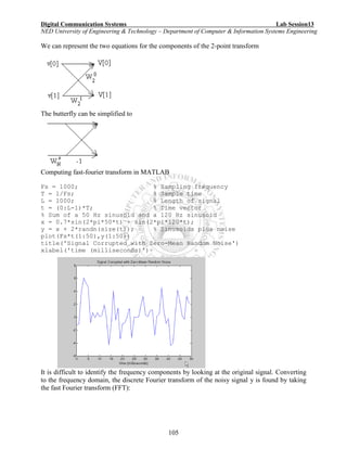
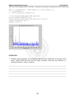
111. Digital Communication Systems Lab Session14
NED University of Engineering & Technology – Department of Computer & Information Systems Engineering
108
Lab Session 14
OBJECT
Working with Wavelets
THEORY
A wavelet is a wave-like oscillation with amplitude that starts out at zero, increases, and then
decreases back to zero. It can typically be visualized as a "brief oscillation" like one might see
recorded by a seismograph or heart monitor.
Wavelet Functions:
Orthogonal wavelet
[PHI,PSI,XVAL] = wavefun('wname',ITER) returns the scaling and wavelet functions on
the points grid XVAL.
Biorthogonal wavelet
[PHI1,PSI1,PHI2,PSI2,XVAL] = wavefun('wname',ITER) returns the scaling and
wavelet functions both for decomposition (PHI1,PSI1) and for reconstruction (PHI2,PSI2).
Complex wavelet
[PSI,XVAL] = wavefun('wname',ITER)
Where the function wavefun returns the approximations of the wavelet function 'wname' and the
associated scaling function, if it exists. The positive integer ITER determines the number of
iterations computed; thus, the refinement of the approximations.
Example:
On the following graph, 10 piecewise linear approximations of the sym4 wavelet obtained after
each iteration of the cascade algorithm are shown.
% Set number of iterations and wavelet name.
iter = 10;
wav = 'sym4';
% Compute approximations of the wavelet function using the
% cascade algorithm.
for i = 1: iter
[phi,psi,xval] = wavefun(wav,i);
plot(xval,psi);
hold on
end
title(['Approximations of the wavelet ',wav, ...
' for 1 to ',num2str(iter),' iterations']);
hold off

112. Digital Communication Systems Lab Session14
NED University of Engineering & Technology – Department of Computer & Information Systems Engineering
109
The value of the variable ‘wav’ can be from sym2 to sym45 for orthogonal wavelets.
EXERCISES
1. Using the above example, write the code for 25 piecewise linear approximations of the sym8
wavelet obtained after each iteration of the cascade algorithm. Attach the plot.
______________________________________________________________________________
______________________________________________________________________________
______________________________________________________________________________
______________________________________________________________________________
______________________________________________________________________________
______________________________________________________________________________
______________________________________________________________________________
______________________________________________________________________________
______________________________________________________________________________
_____________________________________________________________________________

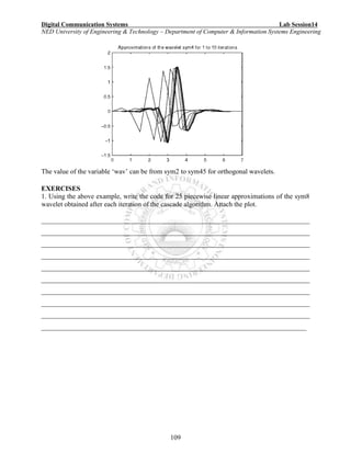
113. Digital Communication Systems Lab Session14
NED University of Engineering & Technology – Department of Computer & Information Systems Engineering
110
2. Referring to the given example, execute the biorthogonal function and give the code below.
[Note: The value of the variable ‘wav’ will be ‘bior’ for biorthogonal functions and the range
must be seen from MATLAB help]
______________________________________________________________________________
______________________________________________________________________________
______________________________________________________________________________
______________________________________________________________________________
______________________________________________________________________________
______________________________________________________________________________
______________________________________________________________________________
______________________________________________________________________________
______________________________________________________________________________
______________________________________________________________________________
______________________________________________________________________________