

![Introduction Gradient Descent Adaptation and Preconditioning Natural Gradient Thoughts
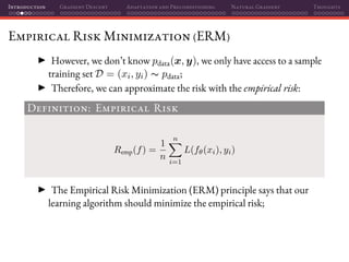
Empirical Risk Minimization (ERM)
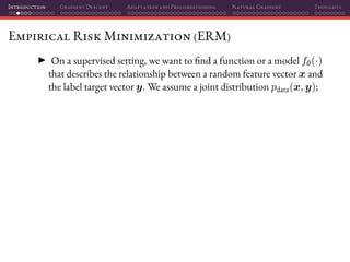
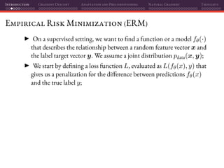
On a supervised setting, we want to find a function or a model fθ(·)
that describes the relationship between a random feature vector x and
the label target vector y. We assume a joint distribution pdata(x, y);
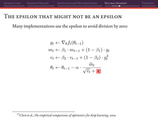
We start by defining a loss function L, evaluated as L(fθ(x), y) that
gives us a penalization for the difference between predictions fθ(x)
and the true label y;
Now, taking the expectation of the loss we have our risk R:
Definition: Risk
R(f) = Ex,y∼pdata
[L(fθ(x), y)
Loss
] = L(fθ(x), y) dpdata(x, y),
that we want to minimize.](https://image.slidesharecdn.com/talkoptimization-201121201106/85/Gradient-based-optimization-for-Deep-Learning-a-short-introduction-11-320.jpg)


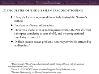
![Introduction Gradient Descent Adaptation and Preconditioning Natural Gradient Thoughts
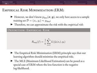
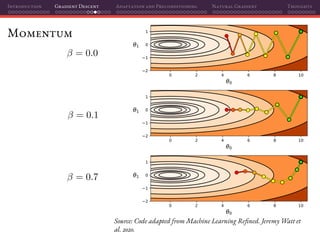
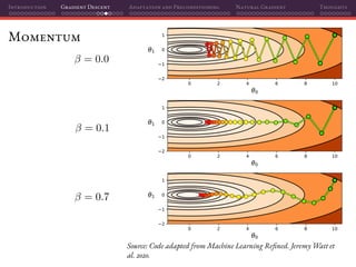
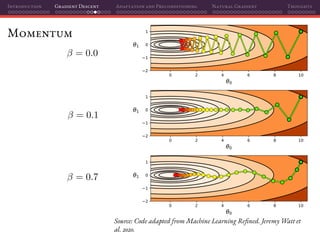
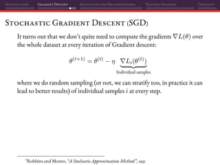
Mini-batch SGD
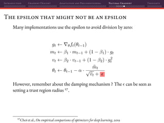
That’s why using mini-batches instead of individual samples on SGD is a
perfect marriage of having better gradient estimates together with improved
parallelization:
L(θ(t)
) =
1
|B|
Batch size
i∈B
Li(θ(t)
)
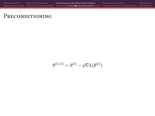
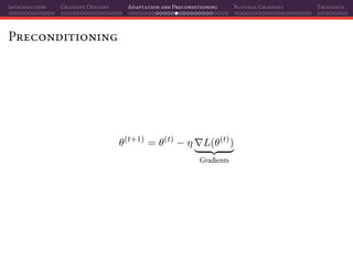
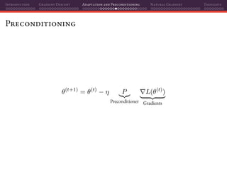
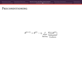
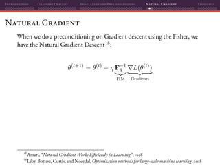
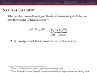
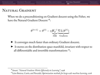
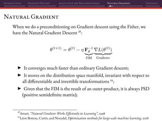
θ(t+1)
= θ(t)
− η L(θ(t)
)
Estimated gradients
If we do random sampling, then:
E[ L(θ(t)
)] = L(θ)
Unbiased estimate](https://image.slidesharecdn.com/talkoptimization-201121201106/85/Gradient-based-optimization-for-Deep-Learning-a-short-introduction-122-320.jpg)


![Introduction Gradient Descent Adaptation and Preconditioning Natural Gradient Thoughts
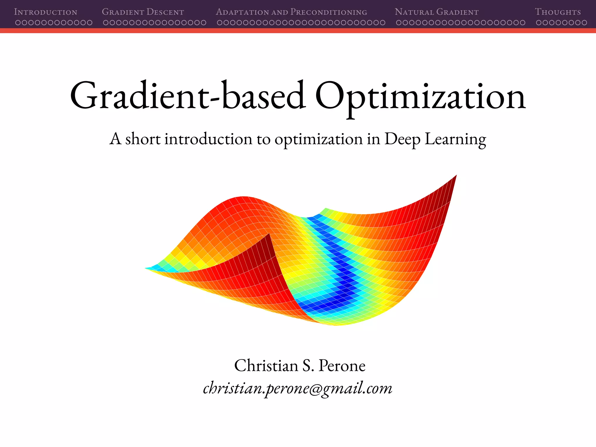
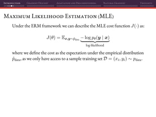
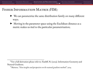
Fisher Information Matrix (FIM)
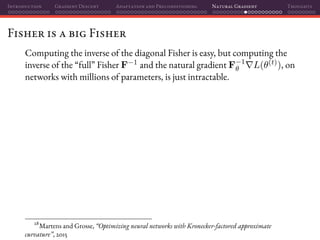
The Fisher Information Matrix is the covariance of the score function
(gradients of the log-likelihood function) with expectation over the model’s
predictive distribution (pay attention to this detail).
Definition: Fisher Information Matrix
Fθ = E
y∼pθ(y|x)
x∼pdata
[ θ log pθ(y|x) θ log pθ(y|x) ]
Where Fθ ∈ Rn×n.](https://image.slidesharecdn.com/talkoptimization-201121201106/85/Gradient-based-optimization-for-Deep-Learning-a-short-introduction-185-320.jpg)
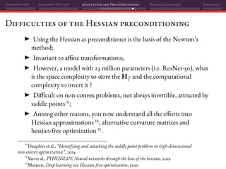
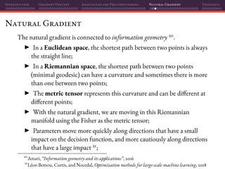
![Introduction Gradient Descent Adaptation and Preconditioning Natural Gradient Thoughts
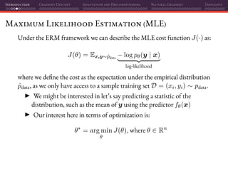
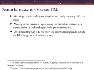
Fisher Information Matrix (FIM)
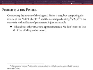
The Fisher Information Matrix is the covariance of the score function
(gradients of the log-likelihood function) with expectation over the model’s
predictive distribution (pay attention to this detail).
Definition: Fisher Information Matrix
Fθ = E
y∼pθ(y|x)
x∼pdata
[ θ log pθ(y|x) θ log pθ(y|x) ]
Where Fθ ∈ Rn×n. We often approximate it using input samples (y is still
from model’s predictive distribution), as we don’t have access to pdata:
Fθ =
1
N
N
i=1
θ log pθ(y|xi) θ log pθ(y|xi)](https://image.slidesharecdn.com/talkoptimization-201121201106/85/Gradient-based-optimization-for-Deep-Learning-a-short-introduction-186-320.jpg)
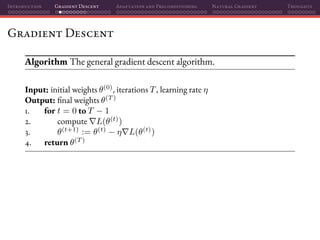
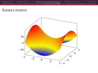
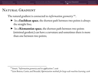
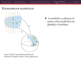
![Introduction Gradient Descent Adaptation and Preconditioning Natural Gradient Thoughts
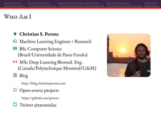
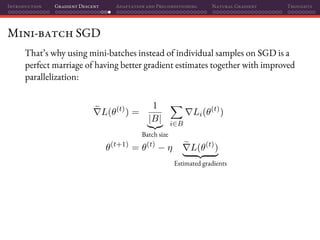
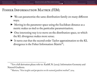
Kullback-Leibler divergence
−20 −15 −10 −5 0 5 10 15 20
KL[P Q] = 5683.243
P
Q](https://image.slidesharecdn.com/talkoptimization-201121201106/85/Gradient-based-optimization-for-Deep-Learning-a-short-introduction-187-320.jpg)
![Introduction Gradient Descent Adaptation and Preconditioning Natural Gradient Thoughts
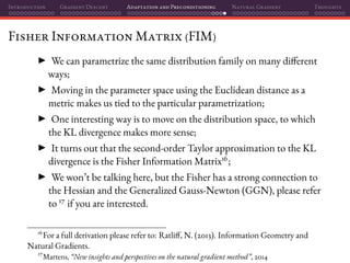
Kullback-Leibler divergence
−20 −15 −10 −5 0 5 10 15 20
KL[P Q] = 3488.456
P
Q](https://image.slidesharecdn.com/talkoptimization-201121201106/85/Gradient-based-optimization-for-Deep-Learning-a-short-introduction-188-320.jpg)
![Introduction Gradient Descent Adaptation and Preconditioning Natural Gradient Thoughts
Kullback-Leibler divergence
−20 −15 −10 −5 0 5 10 15 20
KL[P Q] = 1842.365
P
Q](https://image.slidesharecdn.com/talkoptimization-201121201106/85/Gradient-based-optimization-for-Deep-Learning-a-short-introduction-189-320.jpg)
![Introduction Gradient Descent Adaptation and Preconditioning Natural Gradient Thoughts
Kullback-Leibler divergence
−20 −15 −10 −5 0 5 10 15 20
KL[P Q] = 744.971
P
Q](https://image.slidesharecdn.com/talkoptimization-201121201106/85/Gradient-based-optimization-for-Deep-Learning-a-short-introduction-190-320.jpg)
![Introduction Gradient Descent Adaptation and Preconditioning Natural Gradient Thoughts
Kullback-Leibler divergence
−20 −15 −10 −5 0 5 10 15 20
KL[P Q] = 196.274
P
Q](https://image.slidesharecdn.com/talkoptimization-201121201106/85/Gradient-based-optimization-for-Deep-Learning-a-short-introduction-191-320.jpg)
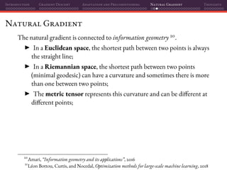
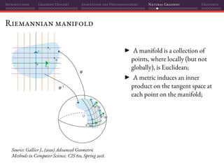
![Introduction Gradient Descent Adaptation and Preconditioning Natural Gradient Thoughts
Kullback-Leibler divergence
−20 −15 −10 −5 0 5 10 15 20
KL[P Q] = 196.274
P
Q](https://image.slidesharecdn.com/talkoptimization-201121201106/85/Gradient-based-optimization-for-Deep-Learning-a-short-introduction-192-320.jpg)
![Introduction Gradient Descent Adaptation and Preconditioning Natural Gradient Thoughts
Kullback-Leibler divergence
−20 −15 −10 −5 0 5 10 15 20
KL[P Q] = 744.971
P
Q](https://image.slidesharecdn.com/talkoptimization-201121201106/85/Gradient-based-optimization-for-Deep-Learning-a-short-introduction-193-320.jpg)
![Introduction Gradient Descent Adaptation and Preconditioning Natural Gradient Thoughts
Kullback-Leibler divergence
−20 −15 −10 −5 0 5 10 15 20
KL[P Q] = 1842.365
P
Q](https://image.slidesharecdn.com/talkoptimization-201121201106/85/Gradient-based-optimization-for-Deep-Learning-a-short-introduction-194-320.jpg)
![Introduction Gradient Descent Adaptation and Preconditioning Natural Gradient Thoughts
Kullback-Leibler divergence
−20 −15 −10 −5 0 5 10 15 20
KL[P Q] = 3488.456
P
Q](https://image.slidesharecdn.com/talkoptimization-201121201106/85/Gradient-based-optimization-for-Deep-Learning-a-short-introduction-195-320.jpg)
![Introduction Gradient Descent Adaptation and Preconditioning Natural Gradient Thoughts
Kullback-Leibler divergence
−20 −15 −10 −5 0 5 10 15 20
KL[P Q] = 5683.243
P
Q](https://image.slidesharecdn.com/talkoptimization-201121201106/85/Gradient-based-optimization-for-Deep-Learning-a-short-introduction-196-320.jpg)


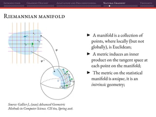
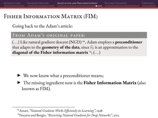
![Introduction Gradient Descent Adaptation and Preconditioning Natural Gradient Thoughts
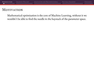
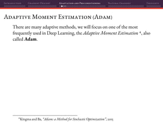
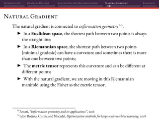
Backpack in PyTorch
If you want to play with K-FAC on PyTorch, you can try using Backpack 29:
from torch import nn
from backpack import backpack, extend
from backpack.extensions import KFAC
from backpack.utils.examples import load_one_batch_mnist
from backpack.utils import kroneckers
X, y = load_one_batch_mnist(batch_size=512)
model = nn.Sequential(
nn.Flatten(),
nn.Linear(784, 10)
)
lossfunc = nn.CrossEntropyLoss()
model = extend(model)
lossfunc = extend(lossfunc)
loss = lossfunc(model(X), y)
with backpack(KFAC(mc_samples=1)):
loss.backward()
named_params = dict(model.named_parameters())
layer_weights = named_params["1.weight"]
# layer_weights.grad = [10, 784]
kfac_f1, kfac_f2 = layer_weights.kfac
# kfac_f1 = [10, 10]
# kfac_f2 = [784, 784]
mat = kroneckers.two_kfacs_to_mat(kfac_f1,
kfac_f2)
# mat = [7840, 7840]
29
Dangel, Kunstner, and Hennig, “BackPACK: Packing more into backprop”, 2019](https://image.slidesharecdn.com/talkoptimization-201121201106/85/Gradient-based-optimization-for-Deep-Learning-a-short-introduction-236-320.jpg)


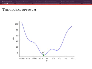
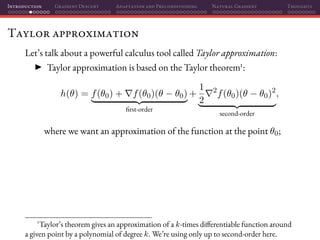
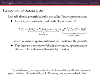
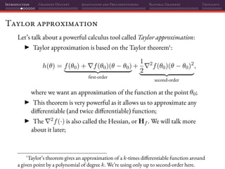
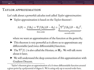
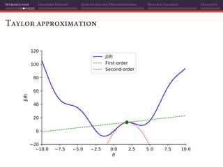
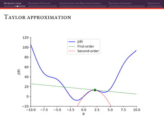
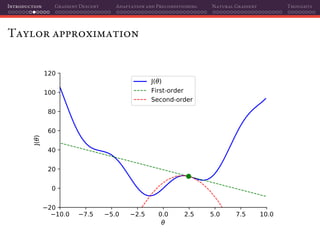
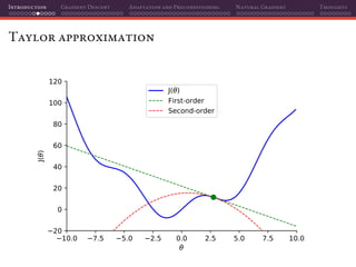
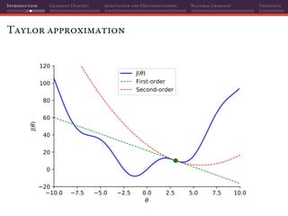
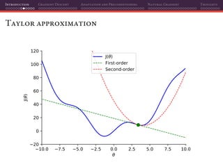
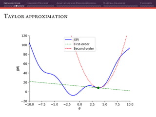
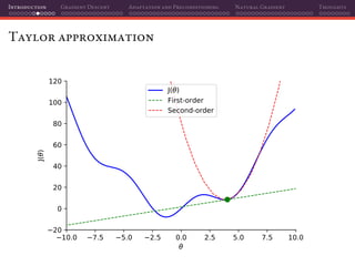
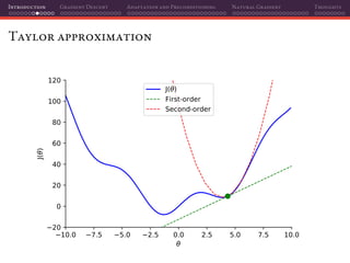
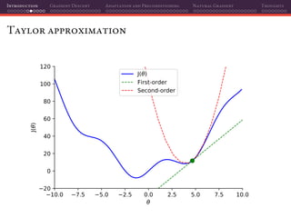
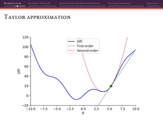
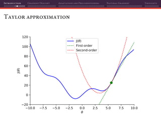
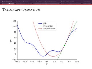
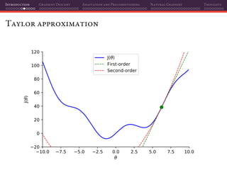
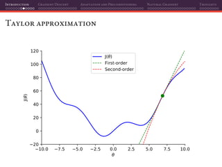
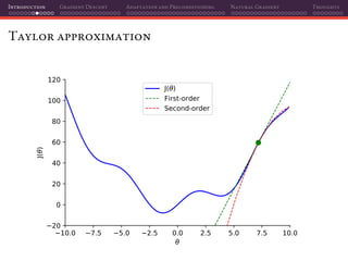
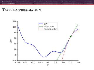
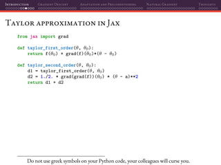
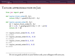
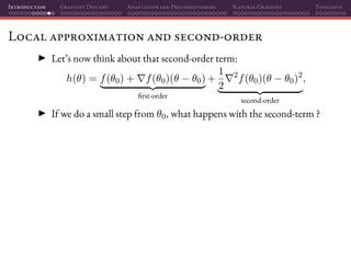
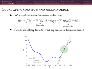
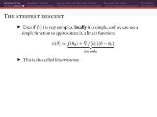
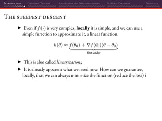
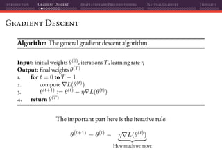
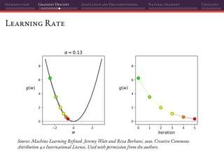
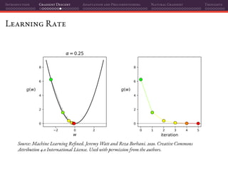
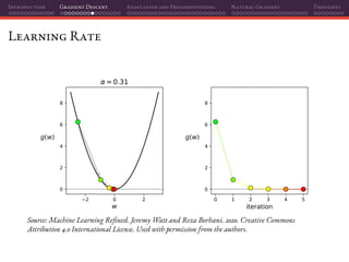
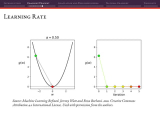
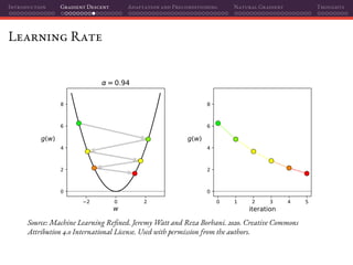
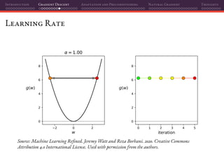
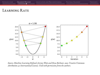
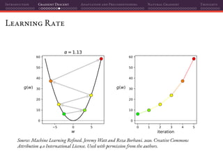
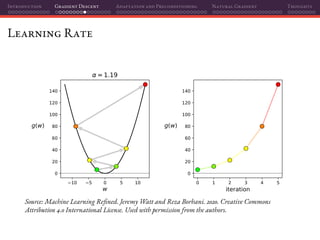
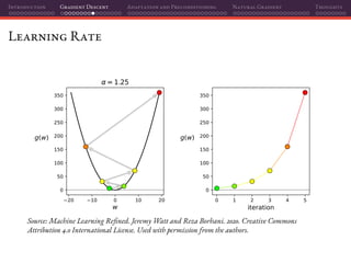
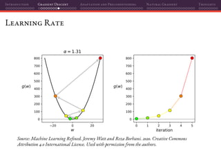
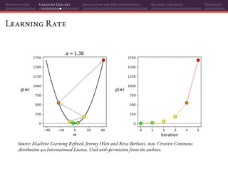
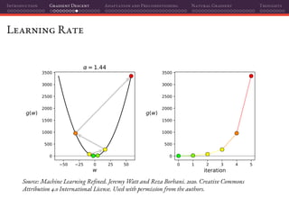
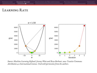
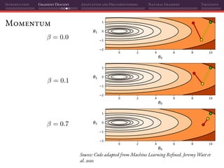
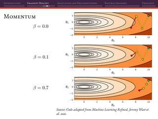
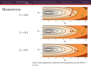
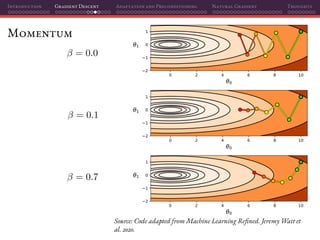
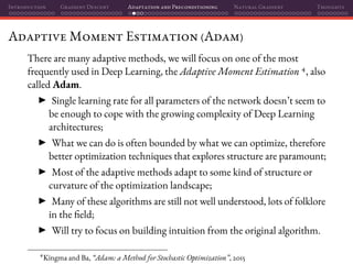
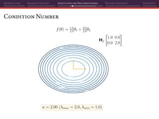
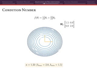
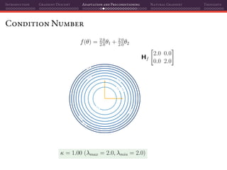
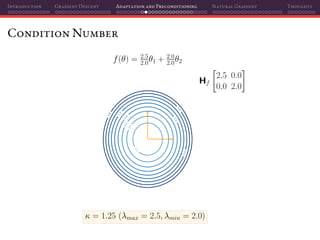
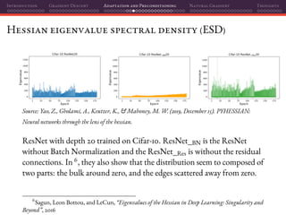
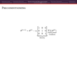
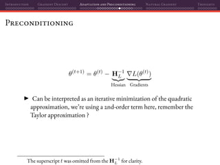
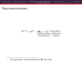
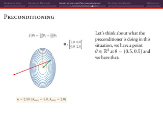
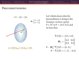
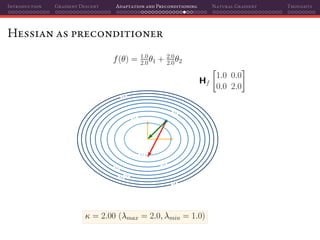
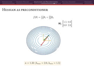
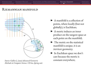
The document discusses gradient descent and its various adaptations and preconditioning techniques, primarily in the context of deep learning optimization. It emphasizes mathematical optimization's role in machine learning for minimizing objective functions and introduces concepts like empirical risk minimization and maximum likelihood estimation. The author also touches on Taylor approximation as an essential calculus tool for optimization within gradient descent methods.


![[Paper Reading] Attention is All You Need](https://cdn.slidesharecdn.com/ss_thumbnails/reading20181228-190111054908-thumbnail.jpg?width=640&height=640&fit=bounds)