A ppt which describes the use of GRADIENT DESCENT algorithm and how it is used to optimise any function. It is shown using various examples.

1. Optimization of Mathematical
Functions Using Gradient Descent
Based Algorithms
REGIONAL INSTITUTE OF EDUCATION
BHUBANESWAR
• BY – SHOVAN PANDA (24282U218035)
• B.SC B.ED 8TH
SEM

2. INTRODUCTION
1.

3. INTRODUCTION
● Optimization aims to maximize or minimize a specified amount under
constraints. Essential for finding suitable solutions to real-world
problems, including maximizing and minimizing functions.
● Gradient Descent is specifically used when the goal is to find the
minimum of a function.
● The function must be differentiable and convex for Gradient Descent to
be applicable.
● Gradient Descent is extensively used in deep learning and machine
learning models for optimizing loss functions.
● Gradient Descent is a first-order iterative optimization algorithm for
differentiable convex functions.

4. LITERATURE REVIEW
2

5. HISTORY OF GRADIENT DESCENT
.
● Gradient descent's origins are in calculus and optimization theory from the
18th and 19th centuries.
● Contributions from Isaac Newton and Joseph-Louis Lagrange in finding
function extrema.
● Formalized as an iterative optimization procedure in the early 20th century.
● Augustin-Louis Cauchy's "method of steepest descent" (1847) is a
precursor.
● Became a standard method in econometrics, statistics, control theory, AI,
and neural networks by the 1960s-70s.
● Interest reignited in the late 20th and early 21st centuries with deep
learning growth.

6. 3
FORMULATION OF
PROBLEM

7. OBJECTIVE
● Gradient descent is an iterative method leading to a function's minimum
(with constraints).
● The core formula for Gradient Descent:
● J(Θ) is the function to optimize, Θ is the parameter.
● The aim is to understand and replicate this formula within a Linear
Regression model.

8. PREDICTION
• A machine learning model tries to make a prediction of a new set of inputs given
a set of known inputs and outputs.
• Error is the difference
between predicted and
actual outputs:

9. COST FUNCTION
● A Loss Function/Cost Function measures the effectiveness of a Machine
Learning Algorithm.
● Loss function computes error for one training example; Cost function
computes the average loss over all training examples.
● For 'N' data points, the Cost function is the total squared error:
• The primary goal of any ML algorithm is to minimize this cost function.
• The cost function often resembles a convex curve like

10. HOW TO MINIMIZE ANY FUNCTION
.
● Intuition: Imagine descending a graph from a 'green' point to a 'red' minimum,
not knowing the destination.
● Gradient Descent uses derivatives to make these decisions rapidly and
efficiently.
● Calculating the tangent line
helps determine the desired
direction to the minima.
● The slope also indicates steepness;
a smaller slope (closer to minimum)
requires fewer steps.

11. LEARNING RATE ()
● Learning Rate (α): A hyperparameter controlling the size of steps and
degree of coefficient change.
● Set by the user and typically
constant throughout the algorithm.
● Optimal Value: Leads to faster
convergence with fewer steps.
● Too High: Algorithm fails to converge,
cost increases.
● Too Low: Convergence is very slow.
● Finding the optimal learning rate is crucial.

12. CALCULATING GRADIENT DESCENT
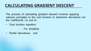
The process of calculating gradient descent involves applying
calculus principles to the cost function to determine derivatives wrt
( ).
the coefficients m and b
• :
Cost function equation
For simplicity
• :
Partial derivatives and

13. CALCULATING GRADIENT DESCENT
Derivative of error wrt ‘m’
(As here X, b and Y are
constants)
Derivative of error wrt ‘m’
(As here m, X and Y are constants)

14. CALCULATING GRADIENT DESCENT
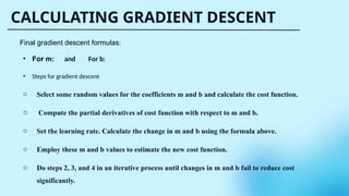
Final gradient descent formulas:
• For m: and For b:
• Steps for gradient descent
o Select some random values for the coefficients m and b and calculate the cost function.
o Compute the partial derivatives of cost function with respect to m and b.
o Set the learning rate. Calculate the change in m and b using the formula above.
o Employ these m and b values to estimate the new cost function.
o Do steps 2, 3, and 4 in an iterative process until changes in m and b fail to reduce cost
significantly.

15. ANALYSIS AND
FINDING
04

16. Function Optimization
• : ( )=
Actual value let f x
0 = -2
The known minimum value of this function is at x
• Experimental demonstration
o 1 :
INPUT () = 0.1 150
Learning rate and iterations
1:
OUTPUT = -2 ( )=0
The algorithm covered to x and f x
59
around the th
iterations
o 2:
INPUT () = 0.01 150
Learning rate and iterations
1:
OUTPUT = -2 ( )=0
The algorithm approached to x and f x
but took more than 150 iterations to converges
fully

17. RESULT
A higher learning rate leads to significantly faster convergence (59
iterations) compared to a lower learning rate (0.01), which takes
many more iterations to reach the minimum. This highlights the critical
importance of turning hyperparameters like the learning rates.

18. APPLICATION OF GRADIENT DESCENT
• Regression analysis: Finding best fit lines/ curves in a data.
• Machine learning / Deep learning:
o Price prediction
o Facial recognition
o Disease prediction
o Recommendation system
o Autonomous driving

19. HYPOTHESIS
• Adaptive learning rates: adjusting the step sizes based on local
curvature improves convergence and stability
• Adaptive rates are crucial for faster, more accurate and stable
traning in deep neutral networks across various fields.