The document discusses Differential Evolution (DE), an evolutionary algorithm for continuous function optimization effective for complex problems like non-differentiable, non-continuous functions that may have multiple local minima. It details the processes of initialization, mutation, recombination, crossover, and selection within the DE framework, emphasizing the algorithm's application in various fields such as engineering and finance. Additionally, the document mentions plans for modifying DE through hybridization with the Spider Monkey Algorithm.

1. Kratika Jain
SAU/AM(M)/01
1

2. Randomly Initialized
vectors
Vectors
2

3. 3
Most vectors are
near global optima

4. DE is an Evolutionary Algorithm.
A stochastic population-based algorithm for continuous function optimization (by Storn
and Price, 1995)
This class also includes Genetic Algorithms, Evolutionary Strategies and Evolutionary
Programming Developed to optimize real parameter, real valued functions.
4

5.  Global optimization is necessary in fields such as engineering, statistics and finance.
Many practical problems have objective functions that are non-differentiable, non-
continuous, non-linear, noisy, flat, multi-dimensional or have many local minima,
constraints or stochasticity
 Such problems are difficult if not impossible to solve analytically
 DE can be used to find approximate solutions to such problems
5

6. MAX
𝑋
𝑀𝐼𝑁
Solutions are represented as vectors of size D with each value taken from some domain.
6

7. We will maintain a population of size NP
7

8. INTIALISTATION
MUTATION
RECOMBINATION/CROSSOVER
SELECTION
8

9. 𝐷𝑖𝑓𝑓𝑒𝑟𝑒𝑛𝑡 𝑣𝑎𝑙𝑢𝑒𝑠 𝑜𝑓 𝑟𝑎𝑛𝑑𝑖,𝑗 0,1 𝑎𝑟𝑒 𝑖𝑛𝑡𝑖𝑎𝑙𝑖𝑠𝑒𝑑 𝑓𝑜𝑟 𝑒𝑎𝑐ℎ 𝑖 𝑎𝑛𝑑 𝑗
9
INTIALISATION

10. 10
INTIALISATION

11. INTIALISTATION
MUTATION
RECOMBINATION/CROSSOVER
SELECTION
11

12.  It is Recombination of Vector Differentials to generate mutant vector
 This explores the search space
 𝑋′𝑖
(𝐺)
= 𝑋 𝑎
(𝐺)
+ 𝐹 𝑋 𝑏
𝐺
− 𝑋𝑐
𝐺
Here 𝑎, 𝑏, 𝑐 is randomly chosen vector different from 𝑖
This mutant vector is constructed through a specific mutation operation based on adding
differences between randomly selected
elements of the population to another element.
12

13. 13(JOURNAL OF GLOBAL OPTIMISATION BY RAINER STORN AND KENNETH PRICE)

14. 14
(Differential Evolution:Foundations, Perspectives, and Applications by Swagatam Das1 and P. N. Suganthan

15.  DE/rand/1/bin
 DE/best/2/bin
 DE/best/1/exp
 DE/current-to-rand/1/exp
15

16. Step-I Step-II
16

17. Step-III Step-IV
17

18. Step-V
18

19. INTIALISTATION
MUTATION
RECOMBINATION/CROSSOVER
SELECTION
19

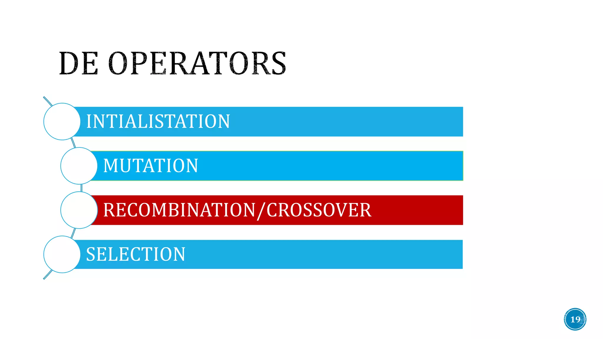
20. Crossover is a genetic operator used to vary the programming of a chromosome
or chromosomes from one generation to the next. It is analogous to reproduction , upon
which genetic algorithms are based.
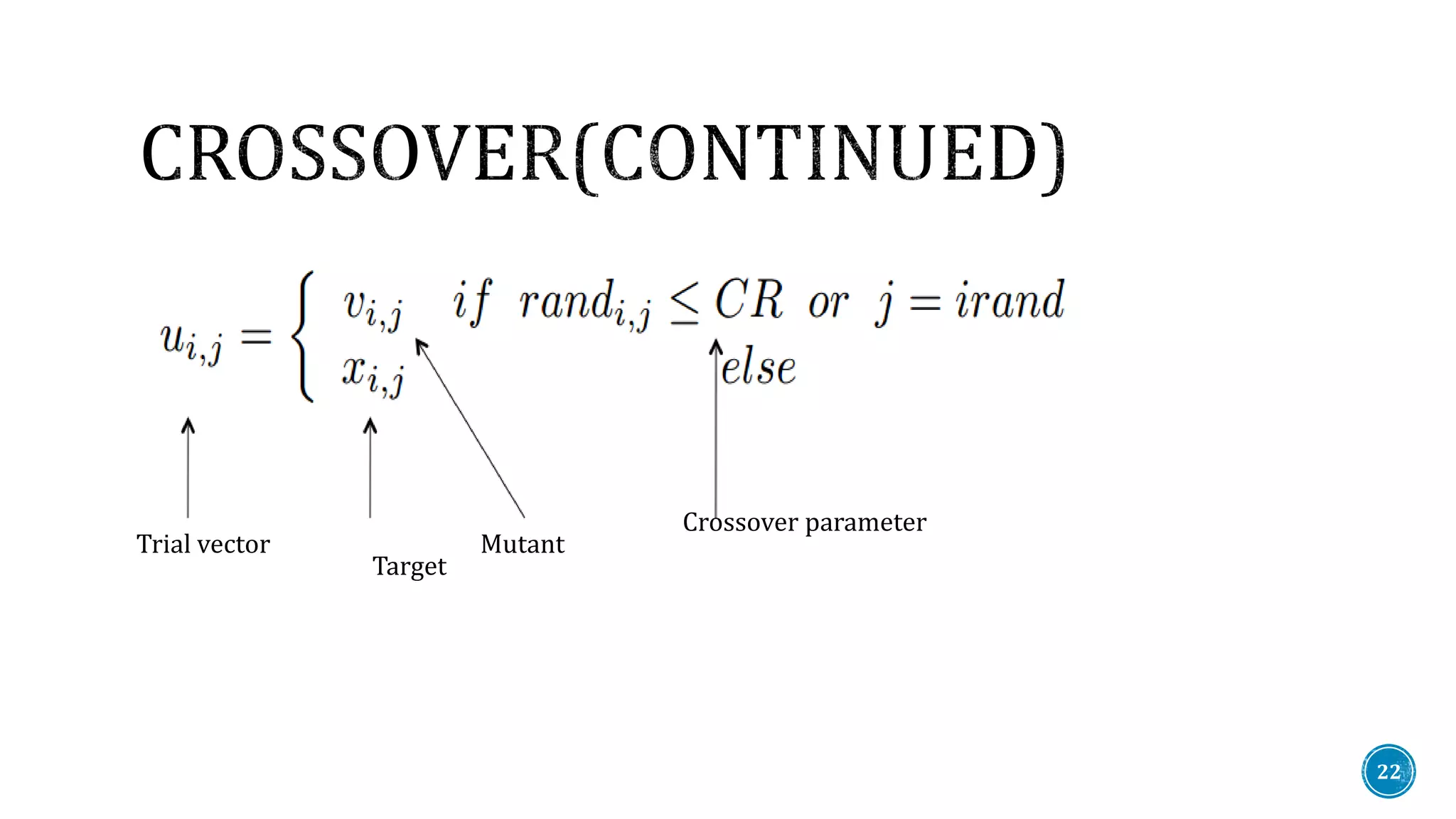
Crossover operator combines components from the current element and from the
mutant vector, according to a control parameter CR ∈ [0, 1].
 It exploits the solution space.
20

21. 21

22. Trial vector
Target
Mutant
Crossover parameter
22

23. NON CONSECUTIVE BINOMIAL CROSSOVER.
CONSECUTIVE EXPONENTIAL CROSSOVER.
CONSECUTIVE BINOMIAL CROSSOVER.
NON CONSECUTIVE EXPONENTIAL CROSSOVER.
23

24.  If the random vector/offspring replicates 𝒗𝒊,𝒏,a randomly chosen parameter of 𝒙𝒊,𝒏, 𝑥𝑖,𝑟,𝑛
will replace the corresponding parameter of the child 𝒄𝒊,𝒏 𝑐𝑖,𝑗,𝑛 .
On the other hand, if 𝒄𝒊,𝒏 inherits no parameter from 𝑣𝑖,𝑛 and hence no evolution happens,
a randomly chosen parameter of the child 𝒄𝒊,𝒏, 𝑐𝑖,𝑗,𝑛,will be replaced by the corresponding
parameter of the mutant 𝒗𝒊,𝒏, 𝑣𝑖,𝑗,𝑛
𝑐𝑖,𝑗,𝑛 = ቊ
𝑣𝑖,𝑗,𝑛
𝑥𝑖,𝑗,𝑛
𝑅𝑎𝑛𝑑(0,1) ≤ 𝐶𝑅
𝑜𝑡ℎ𝑒𝑟𝑤𝑖𝑠𝑒
24

25. Non-consecutive binomial crossover
𝑥𝑖,𝑛
𝑣𝑖,𝑛
𝐵𝑒𝑟𝑛𝑜𝑢𝑙𝑖
𝐸𝑥𝑝𝑒𝑟𝑖𝑚𝑒𝑛𝑡
𝑐𝑖,𝑛
25

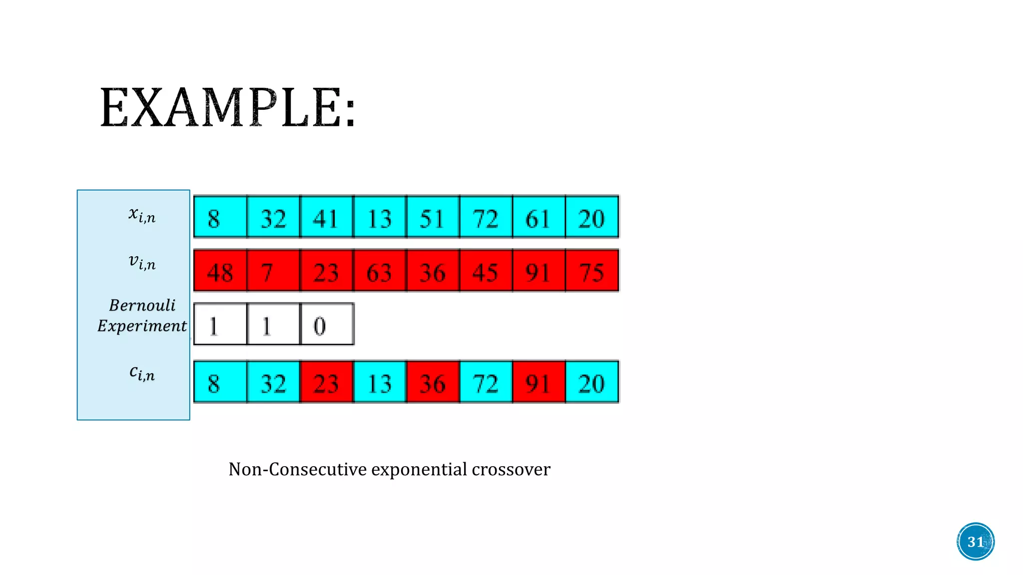
26. In this scheme, an integer 𝑟 is first randomly chosen from [1, 𝑁]. It is the starting point for
exponential crossover.
 𝑐𝑖,𝑟,𝑛 of the offspring 𝒄𝒊,𝒏 is taken from 𝑣𝑖,𝑟,𝑛 of the mutant 𝑣𝑖,𝑛.
 Parameters of the offspring after (in cyclic sense) r depends on a series of
Bernoulli experiments of probability 𝐶𝑟.
The mutant will keep donating its parameters to the offspring until the Bernoulli
experiment is unsuccessful for the first time or the crossover length is already N − 1. The
remaining parameters of the child come from 𝑥𝑖,𝑛
26

27. Consecutive exponential crossover
𝑆𝑡𝑎𝑟𝑡𝑖𝑛𝑔 𝑝𝑜𝑖𝑛𝑡
𝑥𝑖,𝑛
𝑣𝑖,𝑛
𝐵𝑒𝑟𝑛𝑜𝑢𝑙𝑖
𝐸𝑥𝑝𝑒𝑟𝑖𝑚𝑒𝑛𝑡
𝑐𝑖,𝑛
27

28. The number of successful Bernoulli experiment is the crossover length L.
A staring point r is then randomly chosen between 1 and N.
 𝑐𝑖,𝑛inherits L parameters of mutant 𝑣𝑖,𝑛consecutively (in cyclic sense) from the starting
point r (including).
The remaining parameters of 𝑐𝑖,𝑛 come from 𝑥𝑖,𝑛.
28

29. Consecutive binomial crossover
𝑆𝑡𝑎𝑟𝑡𝑖𝑛𝑔 𝑝𝑜𝑖𝑛𝑡
𝑥𝑖,𝑛
𝑣𝑖,𝑛
𝐵𝑒𝑟𝑛𝑜𝑢𝑙𝑖
𝐸𝑥𝑝𝑒𝑟𝑖𝑚𝑒𝑛𝑡
𝑐𝑖,𝑛
29

30. A series of Bernoulli experiments of probability 𝐶𝑟 are carried out in the same way as
described in consecutive exponential crossover.
Used to determine the crossover length L for non-consecutive exponential crossover.
L parameters are randomly chosen from 𝑣𝑖,𝑛 and inherited by 𝑐𝑖,𝑛. 𝑥𝑖,𝑛 donates the
remaining parameters to 𝑐𝑖,𝑛
30

31. Non-Consecutive exponential crossover
𝑥𝑖,𝑛
𝑣𝑖,𝑛
𝐵𝑒𝑟𝑛𝑜𝑢𝑙𝑖
𝐸𝑥𝑝𝑒𝑟𝑖𝑚𝑒𝑛𝑡
𝑐𝑖,𝑛
31

32. INTIALISTATION
MUTATION
RECOMBINATION/CROSSOVER
SELECTION
32

33.  “Survival of the fittest” principle applied in selection
 The trial offspring vector is compared with the target vector and that on
with a better fitness is admitted to the next generation.
33

34. SELECTION
34

35. SELECTION
35

36. Consider the two dimensional function
𝒇 𝒙, 𝒚 = 𝒙 𝟐
+ 𝒚 𝟐
Lets start with 5 candidate solutions randomly initiated in range (-10,10)
• 𝑋1,0=[2,-1]
• 𝑋2,0=[6,1]
• 𝑋3,0=[-3,5]
• 𝑋4,0=[-2,6]
• 𝑋5,0=[6,-7]
For the first vector 𝑿 𝟏,randomly select three other vectors say (randomly) 𝑿 𝟐, 𝑿 𝟒 and 𝑿 𝟓
36

37. The mutant vector is formed as 𝑽 𝟏,𝟎=𝑿 𝟐,𝟎+𝑭.(𝑿 𝟒,𝟎-𝑿 𝟓,𝟎).
The trial offspring vector 𝑈1,0is formed by exchanging components of 𝑉1,0 with the target vector
𝑋1,0.
If we set Cr=0.9
Let rand(0,1)=0.6,since 0.6<0.9, 𝑈1,1,0=𝑉1,1,0 =6+0.8.(-8)=-0.4
Again let rand(0,1)=0.95>0.9
Hence 𝑈1,0=𝑋1,2,0 = −1
The trial(offspring ) is 𝑼 𝟏,𝟎 =
Finally, Fitness of Target(parent)=𝑓 2, −1 = 5
Fitness of Trial(offspring)=𝑓 −0.4, −1 = 1.16
37

38. 38

39. We discuss a simple numerical example to illustrate the DE algorithm
𝑀𝑖𝑛𝑖𝑚𝑖𝑧𝑒 𝑓 𝑥 = 𝑥1 + 𝑥2 + 𝑥3
39

40. Individual 1 Individual 2 Individual 3 Individual 4 Individual 5 Individual 6
𝑥1 0.68 0.92 0.22 0.12 0.40 0.94
𝑥2 0.89 0.92 0.14 0.09 0.81 0.63
𝑥3 0.04 0.33 0.40 0.05 0.83 0.13
𝑓(𝑥) 1.61 2.17 0.76 0.26 2.04 1.70
40

41. Individual
2
Individual
4
Difference
vector
F=0.80 Weighted
D.V
𝑥1 0.92 - 0.12 = 0.80 *0.80 0.64
𝑥2 0.92 - 0.09 = 0.83 *0.80 0.66
𝑥3 0.33 - 0.05 = 0.28 *0.80 0.22
Here Individual 2 and 4 are randomly chosen
41

42. Weighted D.V Individual 6 Mutant Vector
𝑥1 0.64 0.94 1.58
𝑥2 0.66 0.63 1.29
𝑥3 0.22 0.13 0.35
42

43. Target Vector Mutant vector Trial vector
𝑥1 0.68 1.58 1.58
𝑥2 0.89 1.29 0.89
𝑥3 0.04 0.35 0.04
𝑓(𝑥) 1.61 3.22 2.51
Here CR=0.50
43

44. NP = 5 or 10 times of number of parameter in a vector
 If solutions get stuck take F = 0.5 and then increase F or NP
 F∈ [0.4, 1] is very effective range
 CR = 0.9 or 1 for a quick solution
44

45. SUMMARY OF THE ALGORITHM(Taken from:Water Resources Research Report by Vasan Arunachalam) 45

46. [1] R. Storn and K. Price, “Differential evolution – a simple and efficient heuristic for global
optimization over continuous spaces,” J. Glob. Optim., vol. 11, pp. 341–359, 1997.
[2] Swagatam Das1 and P. N. Suganthan2, Differential Evolution:Foundations, Perspectives, and
Applications, SSCI (2011)
[3] Chuan Lin · Anyong Qing · Quanyuan Feng, A comparative study of crossover in differential
evolution, pp. :675–703(2011)
[4] Zaharie, D.: A comparative analysis of crossover algorithms in differential evolution. Proc. Of
2007, pp. 171–181 (2007)
[5] http://www1.icsi.berkeley.edu/~storn/code.html
46

47. I will try to modify the algorithm by hybridization of
Differential Evolution with Spider Monkey algorithm
using some changes in the control parameters.
47

48. 48