Please Subscribe to this Channel for more solutions and lectures http://www.youtube.com/onlineteaching Elementary Statistics Practice Test 3 Practice Test Chapter 6 (Normal Probability Distributions) Chapter 6: Normal Probability Distributions

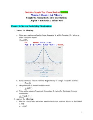
1. 1
Statistics, Sample Test (Exam Review) Solution
Module 3: Chapters 6 & 7 Review
Chapter 6: Normal Probability Distributions
Chapter 7: Estimates & Sample Sizes
Chapter 6: Normal Probability Distributions
1. Answer the following:
a. What percent of normally distributed data value lie within 2 standard deviations to
either side of the mean?
About 95%
Or: Answer: P (-2 < z < 2) =
P (2) – P (-2) = 0.9772 – 0.0228 = 0.9544 or 95.44%
b. For a continuous random variable, the probability of a single value of x is always
Zero (0)
c. The parameters of normal distribution are:
 and  .
d. What are the values of mean and the standard deviation for the standard normal
distribution?
0
 = and 1
 =
2. Answer the following:
a. Find the value of z for a standard normal distribution, such that the area in the left tail
is 0.05
z = –1.645

2. 2
b. Find the value of z for a standard normal distribution, such that the area in the right
tail is 0.1
1 – 0.1 = 0.9 (cumulative area from the left)
1.28 < z < 1.29
z = 1.285
c. Find the following probability: P(z > –0.82)
1 – 0.2061 = 0.7939
d. The z-value for μ of normal distribution curve is always
Zero, why?
e. Usually the normal distribution is used as an approximation to binomial distribution
when np>5, and nq≥5 (In some texts: np > 10, and nq ≥ 10)
3. Find the area of the shaded regions.
a. The graph depicts the standard normal distribution of bone density scores with mean
0 and standard deviation 1.
b. The graph depicts IQ scores of adults, and those scores are normally distributed with
a mean of 100 and a standard deviation of 15.

3. 3
a. b.
a. Answer: p ( Z > − 0.93) = 0.8238
b. 𝑧 =
𝑥− μ
σ
=
106−100
15
= 0.4 & 𝑧 =
𝑥− μ
σ
=
132−100
15
= 2.133
𝑷( 𝟏𝟎𝟔 < 𝒙 < 𝟏𝟑𝟐) = 𝑷( 𝟎. 𝟒 < 𝒁 < 𝟐. 𝟏𝟑𝟑) = 𝟎. 𝟗𝟖𝟑𝟒 ─ 𝟎. 𝟔𝟓𝟓𝟒
= 𝟎. 𝟑𝟐𝟖𝟎 𝑶𝒓 𝟎.𝟑𝟐𝟖𝟏
4. Assume that a randomly selected subject is given a bone density test. Those test scores
are normally distributed with a mean of 0 and a standard deviation of 1.
a. Find the probability that a given score is between −2.13 and 3.77 and draw a sketch
of the region.
Answer: p (− 2.13 < Z < 3.77) = 0.9833
b. Draw a graph and find P19, the 19th percentile. This is the bone density score
separating the bottom 19% from the top 81 %.
Table: 𝑨𝒍 = 𝟎. 𝟏𝟗𝟐𝟐 → 𝒁 =
─ 𝟎. 𝟖𝟕 & 𝑨𝒍 = 𝟎. 𝟏𝟖𝟗𝟒 → 𝒁 =
─ 𝟎. 𝟖𝟖
Answer: ─ 𝟎. 𝟖𝟖 𝒐𝒓 − 𝟎. 𝟖𝟕𝟓

4. 4
5. Three out of eight drinkers acquire the habit by age 20. If 300 drinkers are randomly
selected, using normal approximation to the binomial distribution, find the probability
that:
Given: n = 300, p = 3/8 (0.375),
q = 1 – p = 0.625
a. Exactly 100 acquire the habit by age 20
Binomial Distribution (BD): P(x = 100)
Normal Distribution (ND): P = P ( 99.5 < x < 100.5)
𝜇 = 𝑛𝑝 = 300 (
3
8
) = 112.5
𝜎 = √𝑛𝑝𝑞 = √300 (
3
8
) (
5
8
) = 8.3853
𝑧 =
𝑥 − 𝜇
𝜎
=
99.5 − 112.5
8.3853
= −1.55
𝑧 =
𝑥−𝜇
𝜎
=
100.5−112.5
8.3853
= −1.43
Standard Normal Distribution
(SND):
P(-1.5503 < z < -1.4311) =
0.0764 – 0.0606 = 0.0158
b. At least 125 acquired the habit by age 20
BD: P (x ≥ 125) =
ND: P(x > 124.5) 𝑧 =
𝑥−𝜇
𝜎
=
124.5−112.5
8.3853
= 1.4311

5. 5
SND: =P(z > 1.4311)
= 1 – 0.9236 = 0.0764
c. At most 165 acquired the habit by age 20
BD: P(x ≤ 165) =
ND: P(x < 165.5) 𝑧 =
𝑥−𝜇
𝜎
=
165.5−112.5
8.3853
= 6.3206
above 3.5 in the Z-table
SND: = P(z < 6.3206) =
0.9999
6. IQ scores are normally distributed with a mean of 100 and a standard deviation of 15.
a. What percentage of people has an IQ score above 120?
Given: normal distribution: μ = 100 σ = 15
P(x > 120) 𝑧 =
𝑥−𝜇
𝜎
=
120−100
15
= 1.33
P(x > 120)
= P(z > 1.33) = 1 – 0.9082 =
0.0918,
9.18%
b. What is the maximum IQ score for the bottom 30%?
need to find x when area under the curve corresponds to 0.3
𝑧 =
𝑥 − 𝜇
𝜎
→ 𝑥 = 𝜇 + 𝑍𝜎

6. 6
– 0.53 < z < – 0.52
x = 100 + (– 0.525) ( 15)
= 92.125
maximum IQ score for the bottom
30% is 92.125
7. Men have head breaths that are normally distributed with a mean of 6.0 in and a standard
deviation of 1.0 in.
a. If a man is randomly selected, find the probability that his head breadth is less than 6.2 in.
Given: normal distribution, n = 1, : μ = 6.0 in., σ = 1.0 in.
P( x < 6.2)
𝑧 =
𝑥−𝜇
𝜎
=
6.2−6.0
1
= 0.2
Answer:
P (x < 6.2)
= P (z < 0.2)
= 0.5793
b. If 100 men are randomly selected, find the probability that their head breadth mean
is less than 6.2 in.
Given: n = 100
6.0
x
in
 
= =
/
x
n
 
= = 1.0/√𝟏𝟎𝟎 = 0.1, 𝑧 =
𝑥̅− μ
σ/√𝑛
= 6.2−6.0
0.1 = 2

7. 7
P ( x < 6.2)
= P (z < 2)
= 0.9772
8. The assets (in billions of dollars) of the 4 wealthiest people in a particular country are 33,
29, 16, 11. Assume that samples of size 𝒏 = 𝟐 are randomly selected with
replacement from this population of 4 values.
a. After identifying the 𝟏𝟔 = 𝟐𝟒
different possible samples and finding the mean of each
sample, construct a table representing the sampling distribution of the sample mean. In
the table, values of the sample mean that are the same have been combined.
Answer:
Sample 33,33 33,29 33, 16 33,11 29,33 29,29 29,16 29,11 Continue
𝑥̅ 33 31 24.5 22 31 29 22.5 20 …
𝑝(𝑥
̅̅̅̅̅) 1/16 1/16 1/16 1/16 1/16 1/16 1/16 1/16 …

8. 8
b. Compare the mean of the population to the mean of the sampling distribution of the
sample mean.
Answer: 𝜇 =
∑ 𝑥
𝑁
=
33 + 29 + 16 + 11
4
= 22.25
𝜇𝑥̅ = ∑ 𝑥̅ 𝑃(𝑥̅)
= 33(
1
16
) + 31(
2
16
) + ⋯ + 11(
1
16
) = 22.25
The mean of the population: 𝜇 = 22.25
Is Equal To:
The mean of the sample means: 𝜇𝑥̅ = 22.25
c. Do the sample means target the value of the population mean? In general, do sample
means make good estimates of population means? Why or why not?
Answer:
Yes, the sample means do target the population mean.
In general, sample means make good estimates of population means because the mean is
an unbiased estimator. An unbiased estimator is the one such that the expected value
or the mean of the estimates obtained from samples of a given size is equal to the
parameter being estimated. In this case: 𝜇𝑥̅ = 𝜇 = 22.25
9. The population of current statistics students has ages with mean μ and standard deviation
σ. Samples of statistics students are randomly selected so that there are exactly 44

9. 9
students in each sample. For each sample, the mean age is computed. What does the
central limit theorem tell us about the distribution of those mean ages?
Answer:
𝑛 > 30
→ A sampling distribution of the mean ages can be approximated by a Normal Distribution with mean
𝜇𝑥̅ = 𝜇 and standard devaition
σ
√𝑛
=
σ
√44
10. A boat capsized and sank in a lake. Based on an assumption of a mean weight of 137 lb.,
the boat was rated to carry 50 passengers (so the load limit was 6,850 lb.). After the boat
sank, the assumed mean weight for similar boats was changed from 137 lb. to 170 lb.
a. Assume that a similar boat is loaded with 50 passengers, and assume that the weights of
people are normally distributed with a mean of 174.1 lb. and a standard deviation of 35.1
lb. Find the probability that the boat is overloaded because the 50 passengers have a
mean weight greater than 137 lb.
Given: n = 50, μ = 174.1 σ = 35.1
P(𝑥̅ > 137) =
P (z > – 7.474) =1
𝑧 =
𝑥̅ − μ
σ/√𝑛
=
137 − 174.1
35.1/√50
= −7.474
– 7.471
Answer: Almost 1.0000.

10. 10
b. The boat was later rated to carry only 15 passengers, and the load limit was changed to
2,550 lb. Find the probability that the boat is overloaded because the mean weight of the
passengers is greater than 170 (so that their total weight is greater than the maximum
capacity of 2,550 lb).
Given: n = 15, μ = 174.1 σ = 35.1
P(𝑥̅ > 170) =
𝑧 =
𝑥̅ − μ
σ/√𝑛
=
170 − 174.1
35.1/√15
= −0.4524
P(𝑥̅ > 170) = P (z > – 0.4524) =0.6736 or 0.6772
Technology Answer: 0.6745.
c. Do the new ratings appear to be safe when the boat is loaded with 15 passengers?
Answer: Because there is a high probability of overloading, the new ratings do not
appear to be safe when the boat is loaded with 15 passengers.
11. At an airport, passengers arriving at the security checkpoint have waiting times that are
uniformly distributed between 0 minutes and 10 minutes. All of the different possible
waiting times are equally likely. Find the probability that a randomly selected passenger
has a waiting time of at least 7 minutes.
Given: The total area under the curve = 1.00, 𝒘𝒊𝒅𝒕𝒉 = 𝟏𝟎
Height (the probability) =
1
𝑤𝑖𝑑𝑡ℎ
→ ℎ =
1
10
= 0.1

11. 11
P (wait time of at least 7 min) = P(x ≥ 7) =
= height × width of shaded area in the figure = 0.1 × 3 = 0.3
12. Information regarding standardized tests used for college admittance.
Scores on the SAT test are normally distributed with a mean of 984 and a standard
deviation of 204. 𝜇 = 984, 𝜎 = 204
Scores on the ACT test are normally distributed with a mean of 20.7 and a standard
deviation of 4.3. 𝜇 = 20.7,𝜎 = 4.3
It is assumed that the two tests measure the same aptitude, but use different scales.
a. If a student gets an SAT score that is the 65-percentile, find the actual SAT score
(Whole number).
𝐴𝑙 = 0.65 → 𝑍 = ?
Answer:𝑍 = ? → 𝑆𝐴𝑇𝑥 =? ?
𝑧 =
𝑥 − 𝜇
𝜎
→ 𝑥 = 𝜇 + 𝑍𝜎 →
= 984 + 0.3853(204) = 1062.61
Answer: 1063
b. What would be the equivalent ACT score for this student (1 decimal)?
𝑃𝑟𝑒𝑣𝑖𝑜𝑢𝑠 𝑍 → 𝐴𝐶𝑇 𝑥 = ?
𝑧 =
𝑥 − 𝜇
𝜎
→ 𝑥 = 𝜇 + 𝑍𝜎 = 20.7 + 0.3853(4.3) = 22.36
Answer: 22.4
c. If a student gets an SAT score of 1494, find the equivalent ACT score (1
decimal).
𝑥 = 1494 → 𝑍 → 𝑥 𝑓𝑜𝑟 𝐴𝐶𝑇
𝑧 =
𝑥 − 𝜇
𝜎
=
1494 − 984
204
= 2.5
→ 𝑥 = 20.7 + 2.5(4.3) = 31.45
Answer: 31.5

12. 12
Statistics, Sample Test (Exam Review) Solution
Module 3: Chapters 6 & 7 Review
Chapter 7: Estimates & Sample Sizes
1. Answer the following:
a. True or False: The confidence interval estimate of the population mean is constructed
around the sample mean.
True / 2
x E x Z
n


 = 
b. Estimation means assigning values to a population parameter based on the value of a
Sample Statistic
c. The confidence level is denoted by:
(1 )100%

−
d. The maximum error (margin of error) of the estimate for μ (based on known σ) is:
/ 2
E Z
n


=
e. The parameter(s) of t distribution is (are) degrees of freedom:
df
2. Answer the following:
a. What criteria are required to apply the t distribution to make a confidence interval for
μ?
The sample must be a simple random sample
Either the sample is from a normally distributed population or n ≥ 30
Population Standard Deviation, σ is unknown
b. Find the values for t for a t-distribution with sample size of 20 and a confidence level
of 95%.
degrees of freedom: df = n – 1 = 19, 2.093
t = 
c. Find the values for t for a t-distribution with sample size of 30 and a confidence level
of 90%.
degrees of freedom: n – 1 = 29, 1.699
t = 

13. 13
3. Find the critical chi-square value
a. for 20 degrees of freedom when the area to the left is 0.01
𝑿𝑳
𝟐
= 𝑿𝟎.𝟗𝟗
𝟐
= 8.260
b. for n=30 when the area to the right is 0.9
degrees of freedom: 29
𝑿𝑹
𝟐
= 𝑿𝟎.𝟗
𝟐
= 19.768
4. A statistician is interested in estimating at a 95% confidence level the mean number of
houses sold per month by all real estate agents in a large city. It is known that the
population standard deviation is 1.9.
a. How large a sample should be taken so that the estimate is within 0.65 of the
population mean?
Given: 95% CI, σ = 1.9, E = 0.65
n = [(zα/2 · σ)/E]2

14. 14
n = [(zα/2 · σ)/E]2 =
[(1.96) (1.9)/0.65]2 =
32.82
≈ 33 (Rounded up)
b. Find this 95% confidence interval, if the mean for such sample size is 3.4
x = 3.4, zα/2 = 1.96, E = 0.65
x – E < μ < x + E
3.4 – 0.65 & 3.4+ 0.65 2.75 < μ < 4.05
5. A random sample of 20 female members of a health club showed that they spend on
average 4.5 hours per week doing physical exercise with standard deviation of 0.75 hours
(assume the time spent on exercise for all female members is approximately normally
distributed)
Given: n = 20, x = 4.5 hr & s = 0.75 hr
a. What is the value of the point estimate of the population mean?
point estimate of μ, the population mean is: x = 4.5 hours per week
b. Construct the 98% confidence interval for the mean time spent on physical
exercise of all such females.
x – E < μ < x + E E = tα/2 · (s/√𝒏)
degree of freedom: df = 20 – 1 = 19
CI = 0.98 → α = 0.02 → t α/2 = 2.539
x – E < μ < x + E
E = tα/2 · (s/√𝒏) =
(2.539)(0.75/√𝟐𝟎) = 0.4258 hours
98% CI: x – E < μ < x + E
→ 4.0742 < μ < 4.9258

15. 15
6. Out of 500 randomly selected adults, 300 said they were in favor of the death penalty for
a person convicted of murder.
Given: n = 500, x = 300
a. What is the value of point estimate of the population proportion?
𝑝̂ =
𝑥
𝑛
=
3
5
= 0.6
b. What is the 95% confidence interval for the population proportion?
CI = 0.95 → α = 0.05 z α/2 = 1.96, 𝑞
̂= 1-0.6 = 0.4
E = zα/2 √𝑝̂𝑞
̂ /𝒏 𝑝̂ − 𝐸 < 𝑝 < 𝑝̂ + 𝐸
E = zα/2 √𝑝̂𝑞
̂ /𝒏 =
(1.96)√(𝟎. 𝟔)(𝟎. 𝟒)/𝟓𝟎𝟎 =
0.0429
𝑝̂ − 𝐸 < 𝑝 < 𝑝̂ + 𝐸
0.5571 < p < 0.6429
7. How large a sample is needed to be 99% confident that the margin of error is 0.025, for
percentage of golfers that are left-handed, if we
a. Assume that 15% of the golfers are left-handed, based on a previous study.
Given: E = 0.025, CI = 0.99, z α/2= 2.575, 𝒑
̂ = 0.15
n = (z α/2)2
𝑝̂𝑞
̂ / E2
n = (z α/2)2
𝑝̂𝑞
̂ / E2
n = [(2.575)2
x 0.15 x 0.85] / 0.0252
n = 1352.6475
but rounds up to 1353

16. 16
b. Assume that we have no prior information suggesting a possible value for the
sample proportion.
Assume 𝒑
̂= 𝒒
̂ = 0.5
n = (z α/2)2
𝑝̂𝑞
̂ / E2
→𝒏 =
𝒛𝜶
𝟐
𝟐
(𝟎.𝟐𝟓)
𝑬𝟐 =
[(2.575)2
(0.25)]/(0.025)2
=
2652.25
≈ 2653 (rounded UP to 2653)
8. Given: 30, 80.5, 4.6
n x s
= = = (assume normal population)
a. Find 98% confidence interval for population variance
(𝒏−𝟏)𝒔𝟐
𝑿𝑹
𝟐 < 𝝈𝟐
<
(𝒏−𝟏)𝒔𝟐
𝑿𝑳
𝟐
df = n – 1 = 29 𝑿𝑹
𝟐
= 𝟒𝟗. 𝟓𝟖𝟖 𝑿𝑳
𝟐
= 𝟏𝟒. 𝟐𝟓𝟕
b. Find 98% confidence interval for population standard deviation
It is merely the square root value of part a.
√𝟏𝟐. 𝟑𝟕𝟒𝟖 < 𝝈 < √𝟒𝟑. 𝟎𝟒𝟏𝟑
→ 𝟑. 𝟓𝟏𝟕𝟖 < 𝝈 < 𝟔. 𝟓𝟔𝟎𝟔
Or: √
(𝒏−𝟏)𝒔𝟐
𝑿𝑹
𝟐 < 𝝈 < √
(𝒏−𝟏)𝒔𝟐
𝑿𝑳
𝟐 → √
(𝟐𝟗)(𝟒.𝟔)𝟐
𝟒𝟗.𝟓𝟖𝟖
< 𝝈 < √
(𝟐𝟗)(𝟒.𝟔)𝟐
𝟏𝟒.𝟐𝟓𝟕
→ 𝟑. 𝟓𝟏𝟕𝟖 < 𝝈 < 𝟔. 𝟓𝟔𝟎𝟔
(𝒏−𝟏)𝒔𝟐
𝑿𝑹
𝟐 < 𝝈𝟐
<
(𝒏−𝟏)𝒔𝟐
𝑿𝑳
𝟐 →
(𝟐𝟗)(𝟒.𝟔)𝟐
𝟒𝟗.𝟓𝟖𝟖
< 𝝈𝟐
<
(𝟐𝟗)(𝟒.𝟔)𝟐
𝟏𝟒.𝟐𝟓𝟕
→
𝟏𝟐. 𝟑𝟕𝟒𝟖 < 𝝈𝟐
< 𝟒𝟑. 𝟎𝟒𝟏𝟑