Download as PDF, PPTX

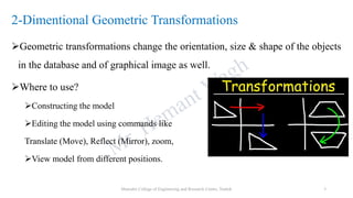


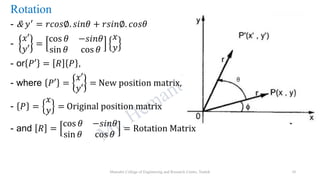


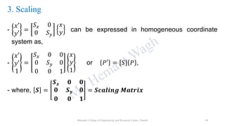


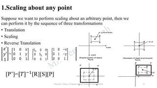


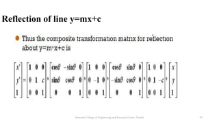


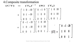
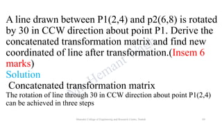


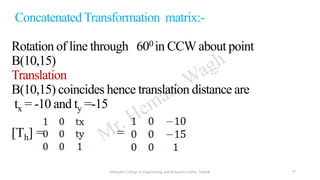

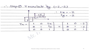


The document discusses various 2D geometric transformations including translation, rotation, scaling, and reflection. It provides the mathematical formulations for each transformation using matrix representations. Translation moves an object by adding a displacement vector. Rotation rotates an object around the origin by a certain angle. Scaling changes the size of an object by multiplying its coordinates by scaling factors. Reflection produces a mirror image of an object across an axis or line.