pp

1. DFT and FFT
• FFT is an algorithm to convert a time domain
signal to DFT efficiently.
• FFT is not unique. Many algorithms are
available.
• Each algorithm has merits and demerits.
• In each algorithm, depending on the sequence
needed at the output, the input is regrouped.
• The groups are decided by the number of
samples.

2. FFTs
• The number of points can be nine too.
• It can be 15 as well.
• Any number in multiples of two integers.
• It can not be any prime number.
• It can be in the multiples of two prime
numbers.

3. FFTs
• The purpose of this series of lectures is to
learn the basics of FFT algorithms.
• Algorithms having number of samples 2N
,
where N is an integer is most preferred.
• 8 point radix-2 FFT by decimation is used
from learning point of view.
• Radix-x: here ‘x’ represents number of
samples in each group made at the first
stage. They are generally equal.
• We shall study radix-2 and radix-3.

4. Radix-2: DIT or, DIF
• Radix-2 is the first FFT algorithm. It was
proposed by Cooley and Tukey in 1965.
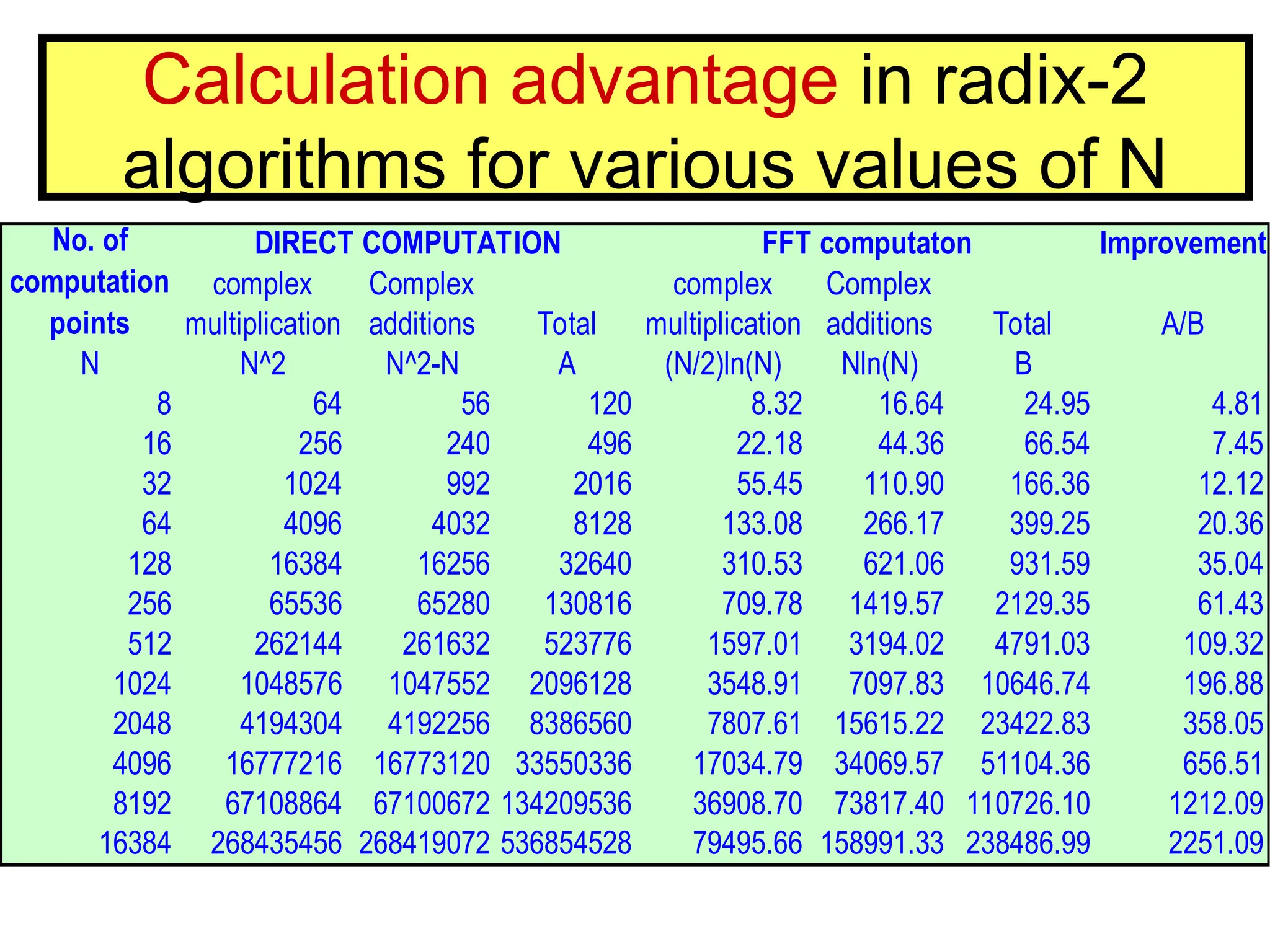
• Though it is not the efficient algorithm, it lays
foundation for time-efficient DFT calculations.
• The next slide shows the saving in time
required for calculations with radix-2.
• The algorithms appear either in
(a) Decimation In Time (DIT), or,
(b) Decimation In Frequency (DIF).
• DIT and DIF, both yield same complexity and
results. They are complementary.
• We shall stress on 8 to radix 2 DIT FFT.

5. Other popular Algorithms
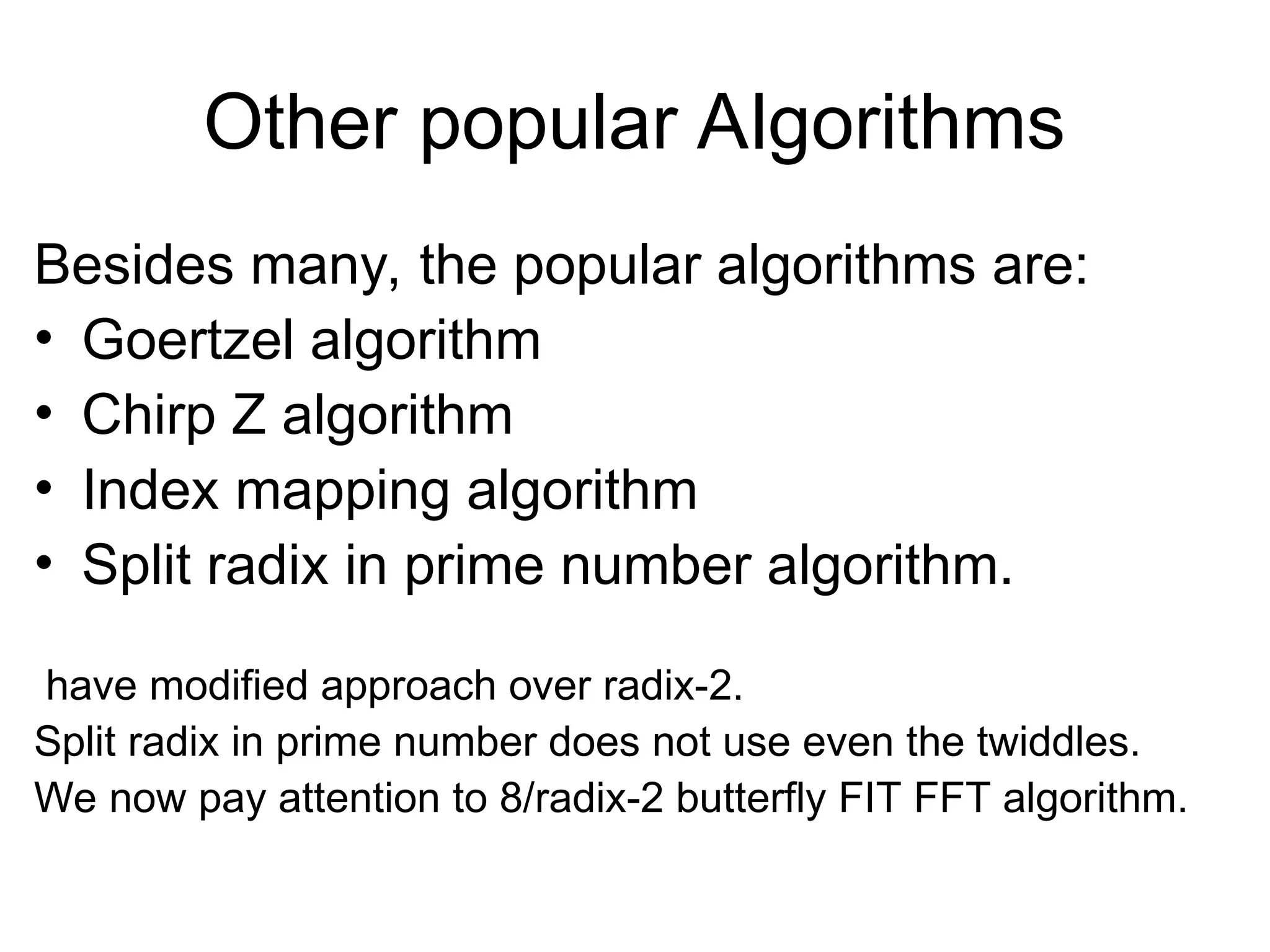
Besides many, the popular algorithms are:
• Goertzel algorithm
• Chirp Z algorithm
• Index mapping algorithm
• Split radix in prime number algorithm.
have modified approach over radix-2.
Split radix in prime number does not use even the twiddles.
We now pay attention to 8/radix-2 butterfly FIT FFT algorithm.

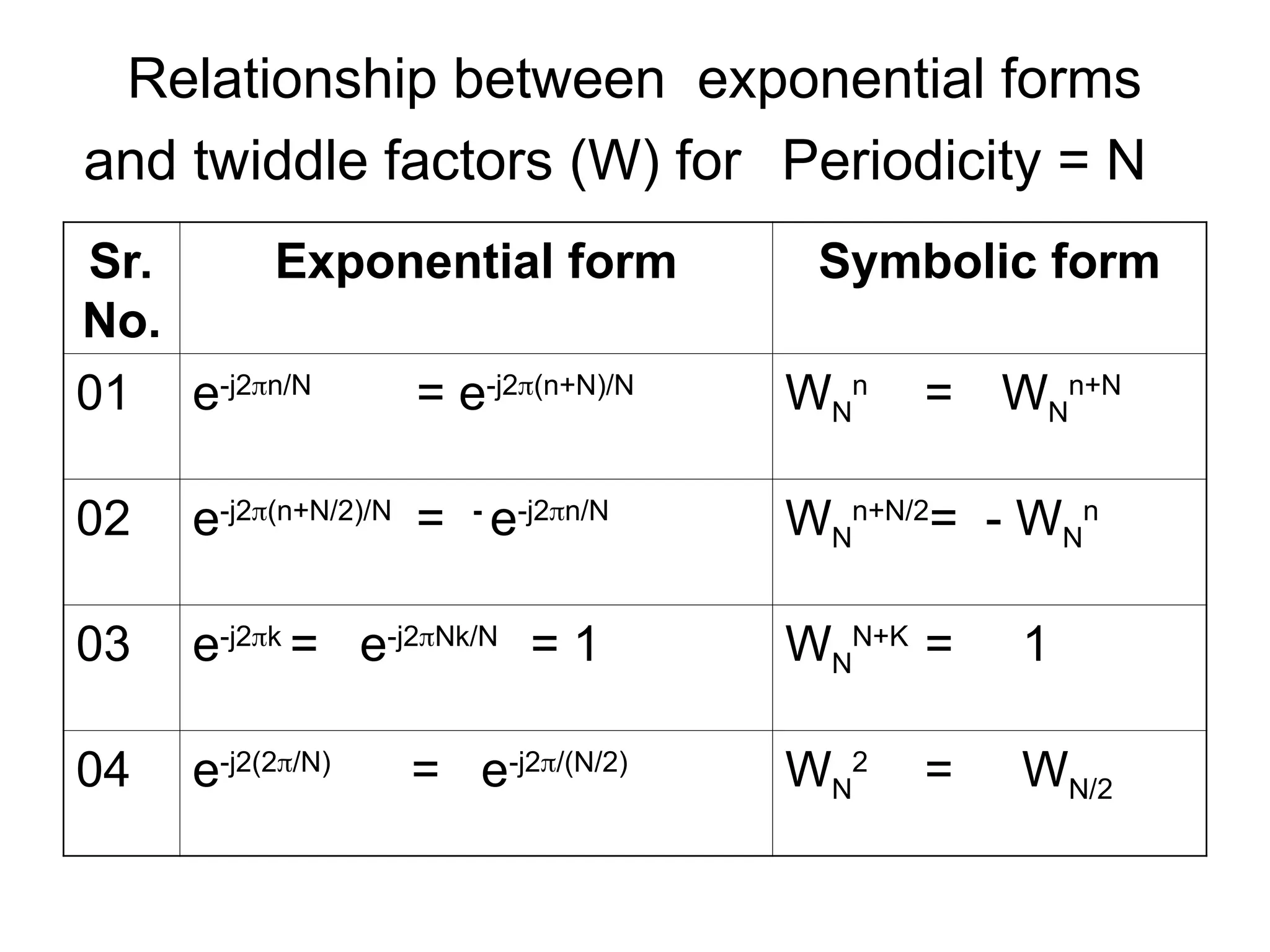
6. Relationship between exponential forms
and twiddle factors (W) for Periodicity = N
Sr.
No.
Exponential form Symbolic form
01 e-j2n/N
= e-j2(n+N)/N
WN
n
= WN
n+N
02 e-j2(n+N/2)/N
= -
e-j2n/N
WN
n+N/2
= - WN
n
03 e-j2k
= e-j2Nk/N
= 1 WN
N+K
= 1
04 e-j2(2/N)
= e-j2/(N/2)
WN
2
= WN/2

7. Values of various twiddles WN
n
for
length N=8
n WN
n
= e(-j2)(n/N)
Remarks
0 1 = 10 WN
0
1 (1-j)/√2 = 1 -45 WN
1
2 -j = 1 -90 WN
2
3 - (1+j)/√2 = 1-135 WN
3
4 -1 = 1 -180 WN
4
= -WN
0
5 - (1-j)/√2 = 1 -225 WN
5
= -WN
1
6 j = 1 90 WN
6
= -WN
2
7 (1+j)/√2 = 1 45 WN
7
= -WN
3

8. DFT calculations
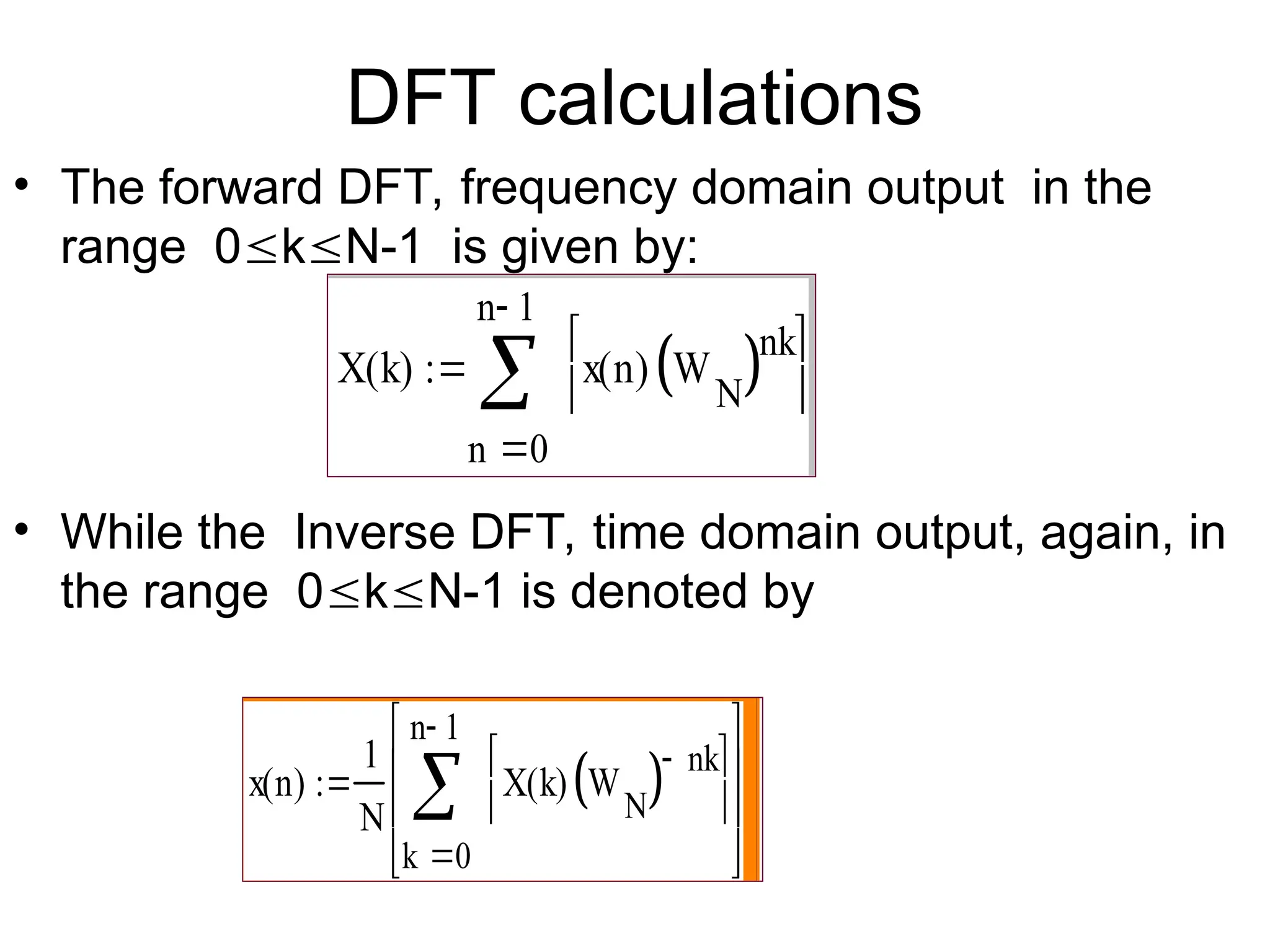
• The forward DFT, frequency domain output in the
range 0kN-1 is given by:
• While the Inverse DFT, time domain output, again, in
the range 0kN-1 is denoted by
X k
( )
0
n 1

n
x n
( ) W
N
 nk







x n
( )
1
N
0
n 1

k
X k
( ) W
N
  nk

















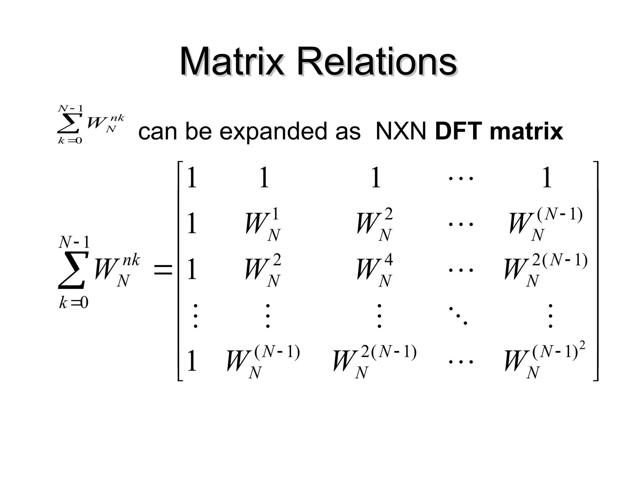
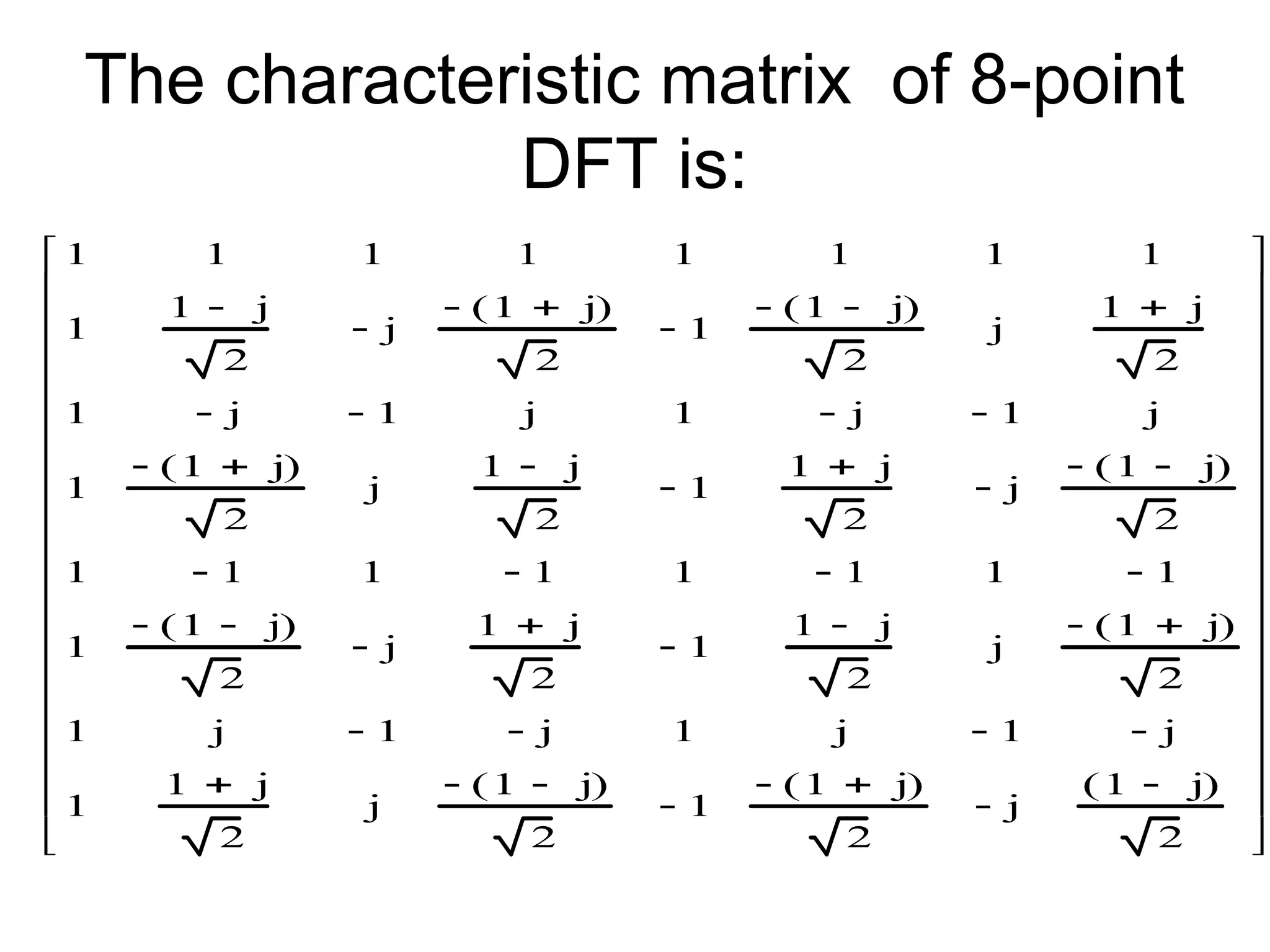
9. Matrix Relations
Matrix Relations
• The DFT samples defined by
can be expressed in NxN matrix as
where
 T
N
X
X
X ]
[
.....
]
[
]
[ 1
1
0 

X
 T
N
x
x
x ]
[
.....
]
[
]
[ 1
1
0 

x
1
0
,
]
[
]
[
1
0







N
k
W
n
x
k
X
N
n
kn
N
   
x(n)
X(k)
1
0
n






 


N
nk
N
W

10. Matrix Relations
Matrix Relations
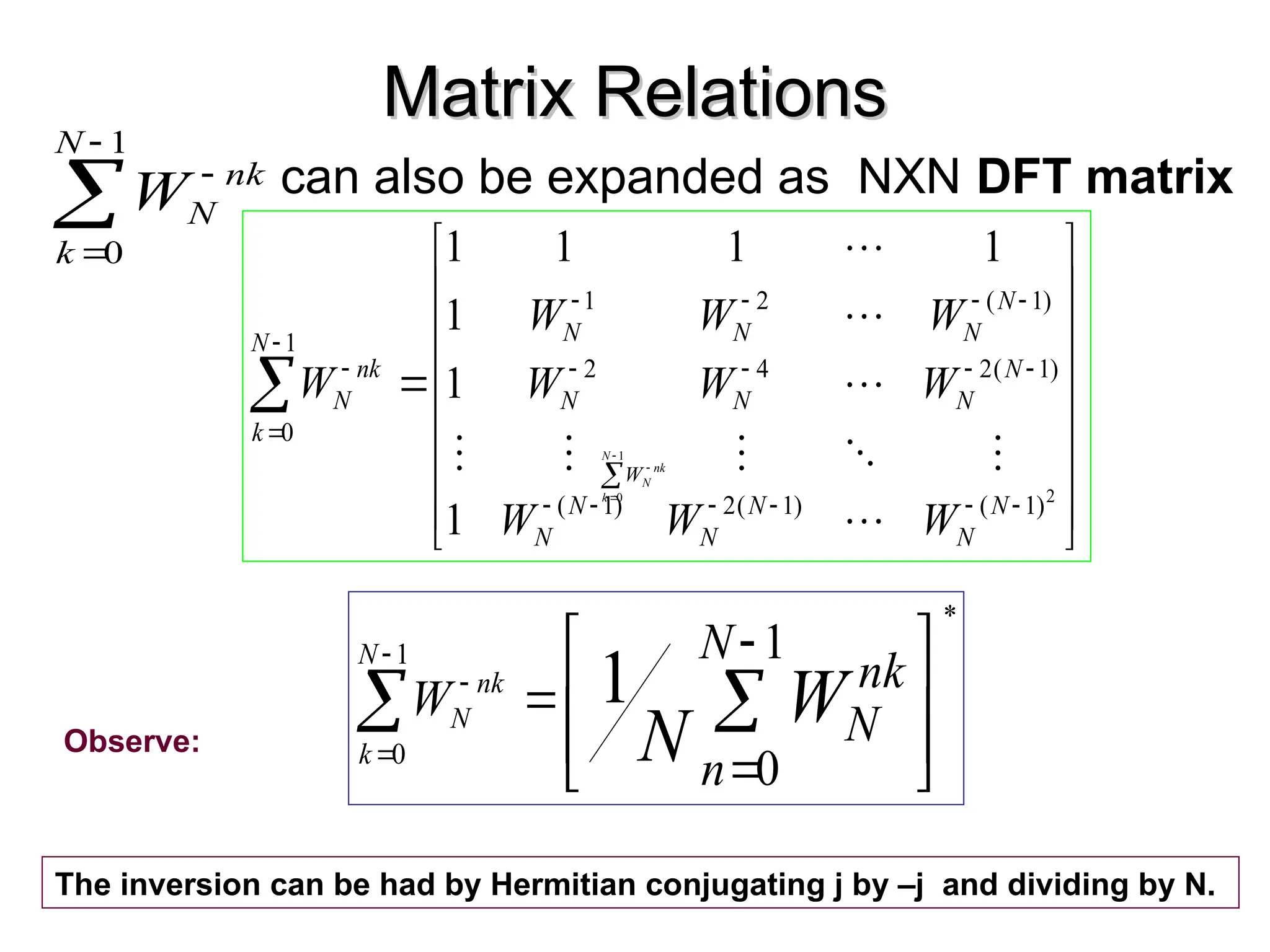
can be expanded as NXN DFT matrix

























2
)
1
(
)
1
(
2
)
1
(
)
1
(
2
4
2
)
1
(
2
1
1
0
1
1
1
1
1
1
1
N
N
N
N
N
N
N
N
N
N
N
N
N
N
N
k
nk
N
W
W
W
W
W
W
W
W
W
W












1
0
N
k
nk
N
W

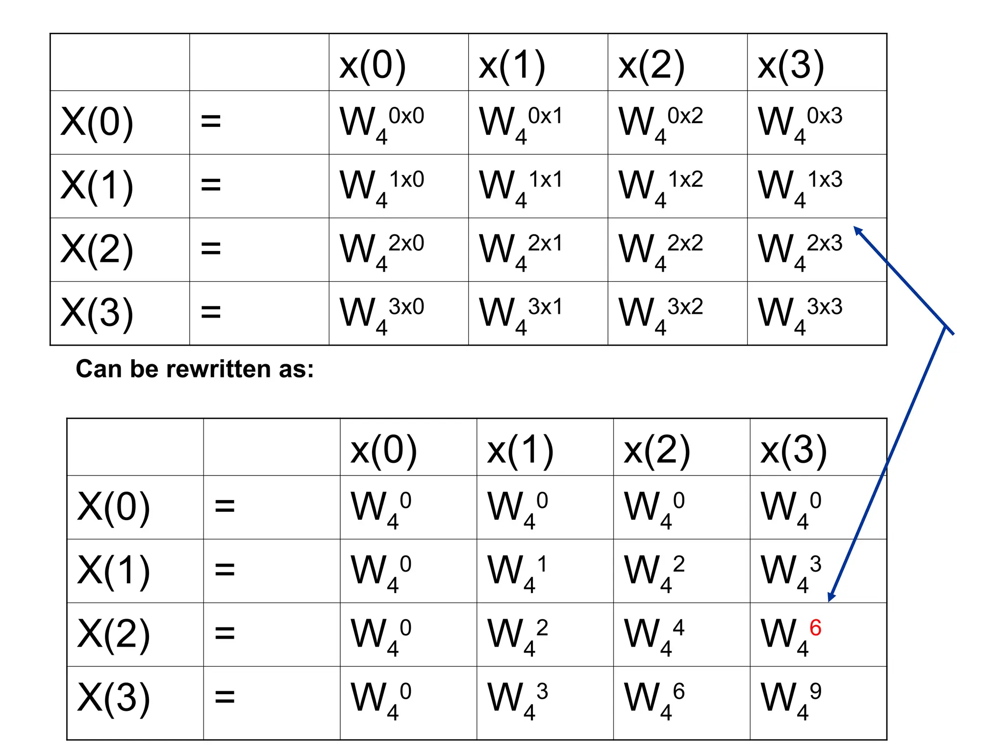
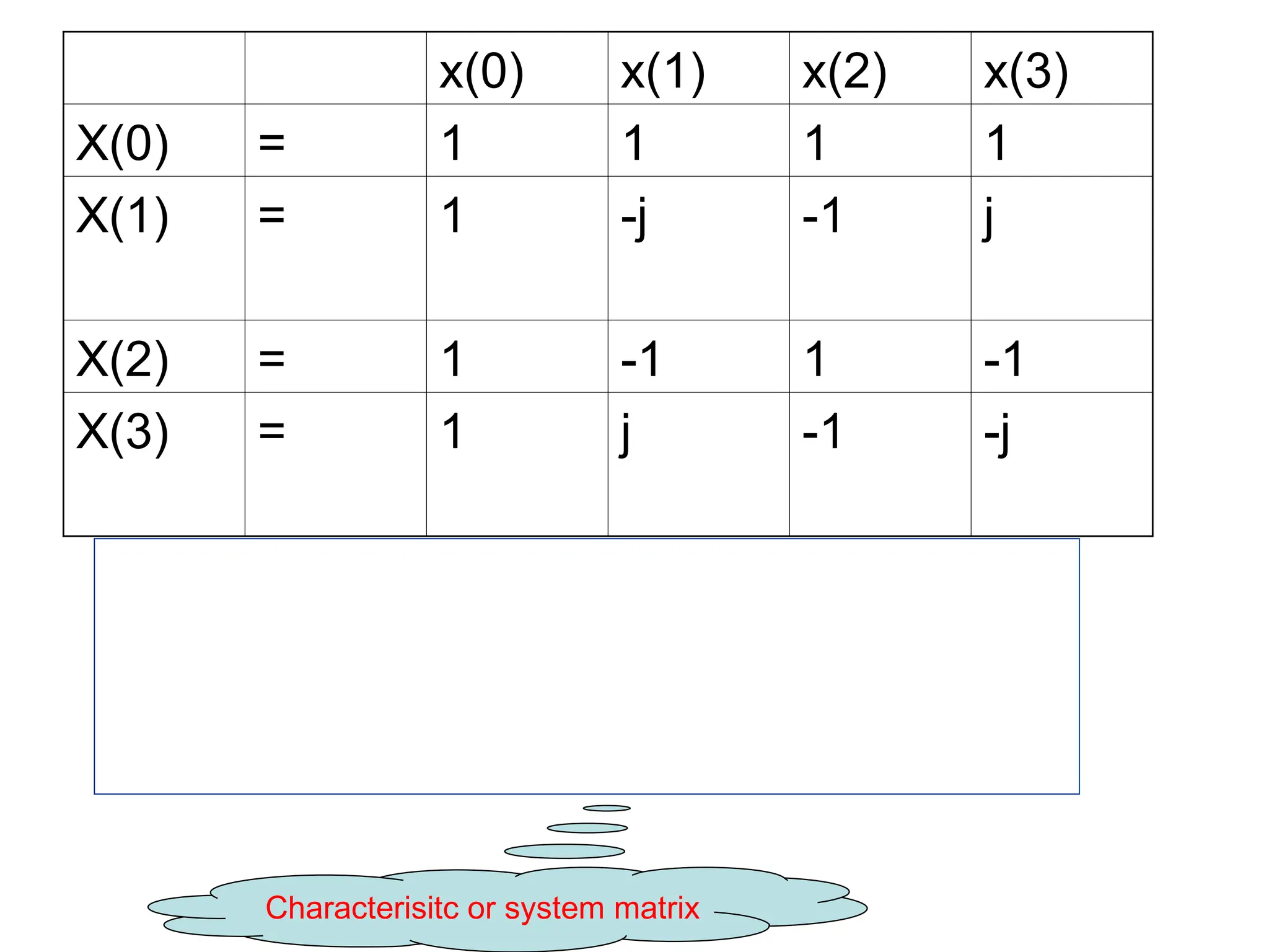
11. DFT:
For N of length 4,range of n, k = [0 1 2 3] each.
Hence X(n) = x(0)WN
n.0
+x(1)WN
n.1
+x(2)WN
n.2
+ x(3)WN
n.3
X k
( )
0
n 1

n
x n
( ) W
N
 nk






 x
x(0) x(1) x(2) x(3)
X(0) = W4
0x0
W4
0x1
W4
0x2
W4
0x3
X(1) = W4
1x0
W4
1x1
W4
1x2
W4
1x3
X(2) = W4
2x0
W4
2x1
W4
2x2
W4
2x3
X(3) = W4
3x0
W4
3x1
W4
3x2
W4
3x3

12. x(0) x(1) x(2) x(3)
X(0) = W4
0x0
W4
0x1
W4
0x2
W4
0x3
X(1) = W4
1x0
W4
1x1
W4
1x2
W4
1x3
X(2) = W4
2x0
W4
2x1
W4
2x2
W4
2x3
X(3) = W4
3x0
W4
3x1
W4
3x2
W4
3x3
x(0) x(1) x(2) x(3)
X(0) = W4
0
W4
0
W4
0
W4
0
X(1) = W4
0
W4
1
W4
2
W4
3
X(2) = W4
0
W4
2
W4
4
W4
6
X(3) = W4
0
W4
3
W4
6
W4
9
Can be rewritten as:

13. x(0) x(1) x(2) x(3)
X(0) = W4
0
W4
0
W4
0
W4
0
X(1) = W4
0
W4
1
W4
2
W4
3
X(2) = W4
0
W4
2
W4
4
W4
6
X(3) = W4
0
W4
3
W4
6
W4
9
x(0) x(1) x(2) x(3)
X(0) = W4
0
W4
0
W4
0
W4
0
X(1) = W4
0
W4
1
W4
2
-W4
1
X(2) = W4
0
W4
2
W4
0
W4
2
X(3) = W4
0
-W4
1
W4
2
W4
1

14. x(0) x(1) x(2) x(3)
X(0) = W4
0
W4
0
W4
0
W4
0
X(1) = W4
0
W4
1
W4
2
-W4
1
X(2) = W4
0
W4
2
W4
0
W4
2
X(3) = W4
0
-W4
1
W4
2
W4
1
x(0) x(1) x(2) x(3)
X(0) = 1 1 1 1
X(1) = 1 -j -1 j
X(2) = 1 -1 1 -1
X(3) = 1 j -1 -j

15. Matrix Relations
Matrix Relations
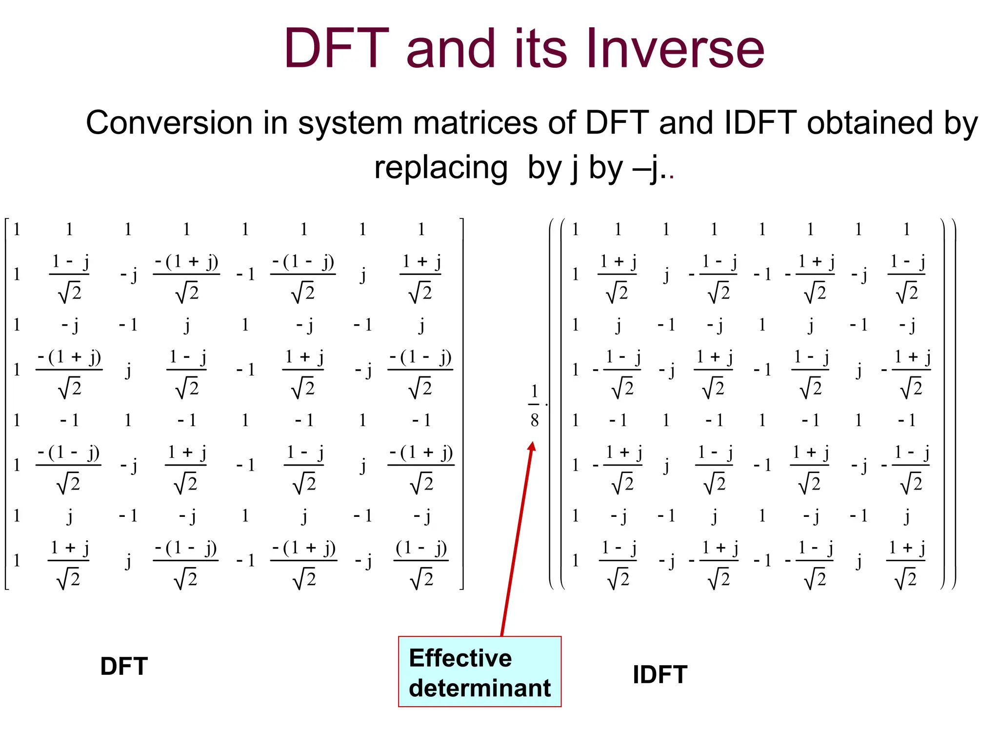
• Likewise, the IDFT is
can be expressed in NxN matrix form as
1
0
,
]
[
]
[
1
0








N
n
W
k
X
n
x
N
k
n
k
N
   
X(k)
1
0
n
x
1











N
n
nk
N
W

16. Matrix Relations
Matrix Relations
can also be expanded as NXN DFT matrix



































2
)
1
(
)
1
(
2
)
1
(
)
1
(
2
4
2
)
1
(
2
1
1
0
1
1
1
1
1
1
1
N
N
N
N
N
N
N
N
N
N
N
N
N
N
N
k
nk
N
W
W
W
W
W
W
W
W
W
W













1
0
N
k
nk
N
W
Observe:




1
0
N
k
nk
N
W














1
0
1
*
1
0
N
n
nk
N
W W
N
N
k
nk
N
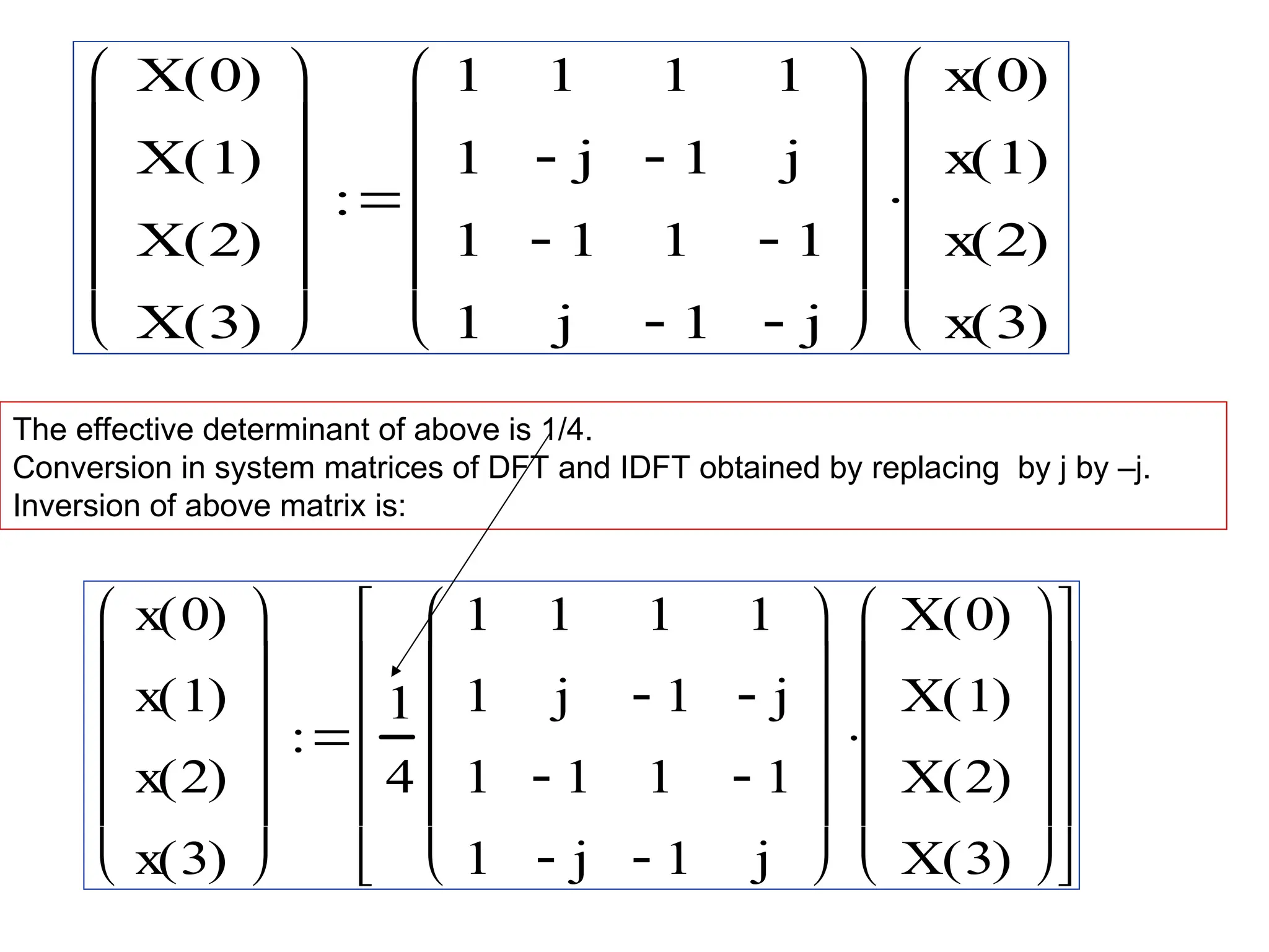
The inversion can be had by Hermitian conjugating j by –j and dividing by N.

17. x(0) x(1) x(2) x(3)
X(0) = 1 1 1 1
X(1) = 1 -j -1 j
X(2) = 1 -1 1 -1
X(3) = 1 j -1 -j
X 0
( )
X 1
( )
X 2
( )
X 3
( )












1
1
1
1
1
j

1

j
1
1

1
1

1
j
1

j













x 0
( )
x 1
( )
x 2
( )
x 3
( )














Characterisitc or system matrix

18. X 0
( )
X 1
( )
X 2
( )
X 3
( )












1
1
1
1
1
j

1

j
1
1

1
1

1
j
1

j













x 0
( )
x 1
( )
x 2
( )
x 3
( )














x 0
( )
x 1
( )
x 2
( )
x 3
( )




1
4
1
1
1
1
1
j
1

j

1
1

1
1

1
j

1

j




X 0
( )
X 1
( )
X 2
( )
X 3
( )










x
The effective determinant of above is 1/4.
Conversion in system matrices of DFT and IDFT obtained by replacing by j by –j.
Inversion of above matrix is:
x 0
( )
x 1
( )
x 2
( )
x 3
( )












1
4
1
1
1
1
1
j
1

j

1
1

1
1

1
j

1

j












X 0
( )
X 1
( )
X 2
( )
X 3
( )



























19. FOR 8 point DFT: N=8
• The system Matrix is:
W8
0x0
W8
0x1
W8
0x2
W8
0x3
W8
0x4
W8
0x5
W8
0x6
W8
0x7
W8
1x0
W8
1x1
W8
1x2
W8
1x3
W8
1x4
W8
1x5
W8
1x6
W8
1x7
W8
2x0
W8
2x1
W8
2x2
W8
2x3
W8
2x4
W8
2x5
W8
2x6
W8
2x7
W8
3x0
W8
3x1
W8
3x2
W8
3x3
W8
3x4
W8
3x5
W8
3x6
W8
3x7
W8
4x0
W8
4x1
W8
4x2
W8
4x3
W8
4x4
W8
4x5
W8
4x6
W8
4x7
W8
5x0
W8
5x1
W8
5x2
W8
5x3
W8
5x4
W8
5x5
W8
5x6
W8
5x7
W8
6x0
W8
6x1
W8
6x2
W8
6x3
W8
6x4
W8
6x5
W8
6x6
W8
6x7
W8
7x0
W8
7x1
W8
7x2
W8
7x0
W8
7x4
W8
7x5
W8
7x6
W8
7x7

20. The characteristic matrix of 8-point
DFT is:
1
1
1
1
1
1
1
1
1
1 j

2
j

1 j

( )

2
1

1 j

( )

2
j
1 j

2
1
j

1

j
1
j

1

j
1
1 j

( )

2
j
1 j

2
1

1 j

2
j

1 j

( )

2
1
1

1
1

1
1

1
1

1
1 j

( )

2
j

1 j

2
1

1 j

2
j
1 j

( )

2
1
j
1

j

1
j
1

j

1
1 j

2
j
1 j

( )

2
1

1 j

( )

2
j

1 j

( )
2



































21. DFT and its Inverse
Conversion in system matrices of DFT and IDFT obtained by
replacing by j by –j..
1
1
1
1
1
1
1
1
1
1 j

2
j

1 j

( )

2
1

1 j

( )

2
j
1 j

2
1
j

1

j
1
j

1

j
1
1 j

( )

2
j
1 j

2
1

1 j

2
j

1 j

( )

2
1
1

1
1

1
1

1
1

1
1 j

( )

2
j

1 j

2
1

1 j

2
j
1 j

( )

2
1
j
1

j

1
j
1

j

1
1 j

2
j
1 j

( )

2
1

1 j

( )

2
j

1 j

( )
2


































1
8
1
1
1
1
1
1
1
1
1
1 j

2
j
1 j

2

1

1 j

2

j

1 j

2
1
j
1

j

1
j
1

j

1
1 j

2

j

1 j

2
1

1 j

2
j
1 j

2

1
1

1
1

1
1

1
1

1
1 j

2

j
1 j

2
1

1 j

2
j

1 j

2

1
j

1

j
1
j

1

j
1
1 j

2
j

1 j

2

1

1 j

2

j
1 j

2





































































DFT IDFT
Effective
determinant

22. Calculation advantage in radix-2
algorithms for various values of N
Improvement
A/B
N N^2 N^2-N A (N/2)ln(N) Nln(N) B
8 64 56 120 8.32 16.64 24.95 4.81
16 256 240 496 22.18 44.36 66.54 7.45
32 1024 992 2016 55.45 110.90 166.36 12.12
64 4096 4032 8128 133.08 266.17 399.25 20.36
128 16384 16256 32640 310.53 621.06 931.59 35.04
256 65536 65280 130816 709.78 1419.57 2129.35 61.43
512 262144 261632 523776 1597.01 3194.02 4791.03 109.32
1024 1048576 1047552 2096128 3548.91 7097.83 10646.74 196.88
2048 4194304 4192256 8386560 7807.61 15615.22 23422.83 358.05
4096 16777216 16773120 33550336 17034.79 34069.57 51104.36 656.51
8192 67108864 67100672 134209536 36908.70 73817.40 110726.10 1212.09
16384 268435456 268419072 536854528 79495.66 158991.33 238486.99 2251.09
No. of
computation
points
DIRECT COMPUTATION FFT computaton
complex
multiplication
Complex
additions
complex
multiplication
Complex
additions
Total Total

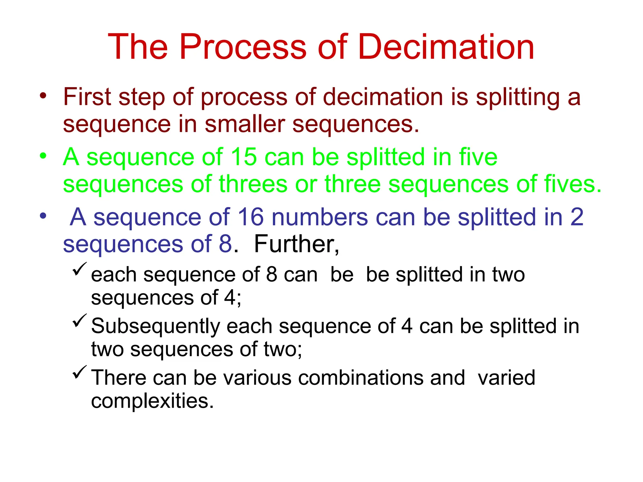
23. The Process of Decimation
• First step of process of decimation is splitting a
sequence in smaller sequences.
• A sequence of 15 can be splitted in five
sequences of threes or three sequences of fives.
• A sequence of 16 numbers can be splitted in 2
sequences of 8. Further,
each sequence of 8 can be be splitted in two
sequences of 4;
Subsequently each sequence of 4 can be splitted in
two sequences of two;
There can be various combinations and varied
complexities.

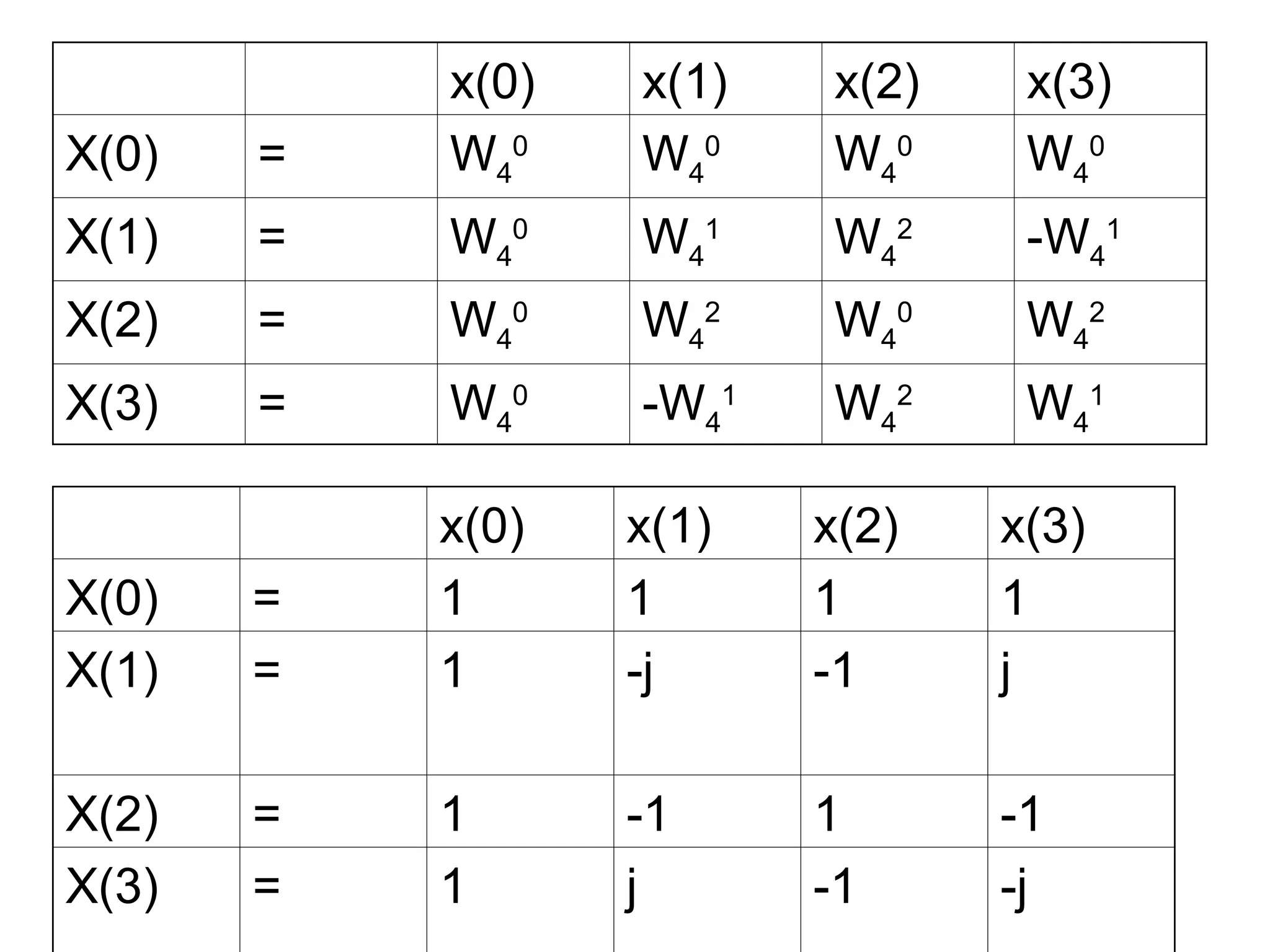
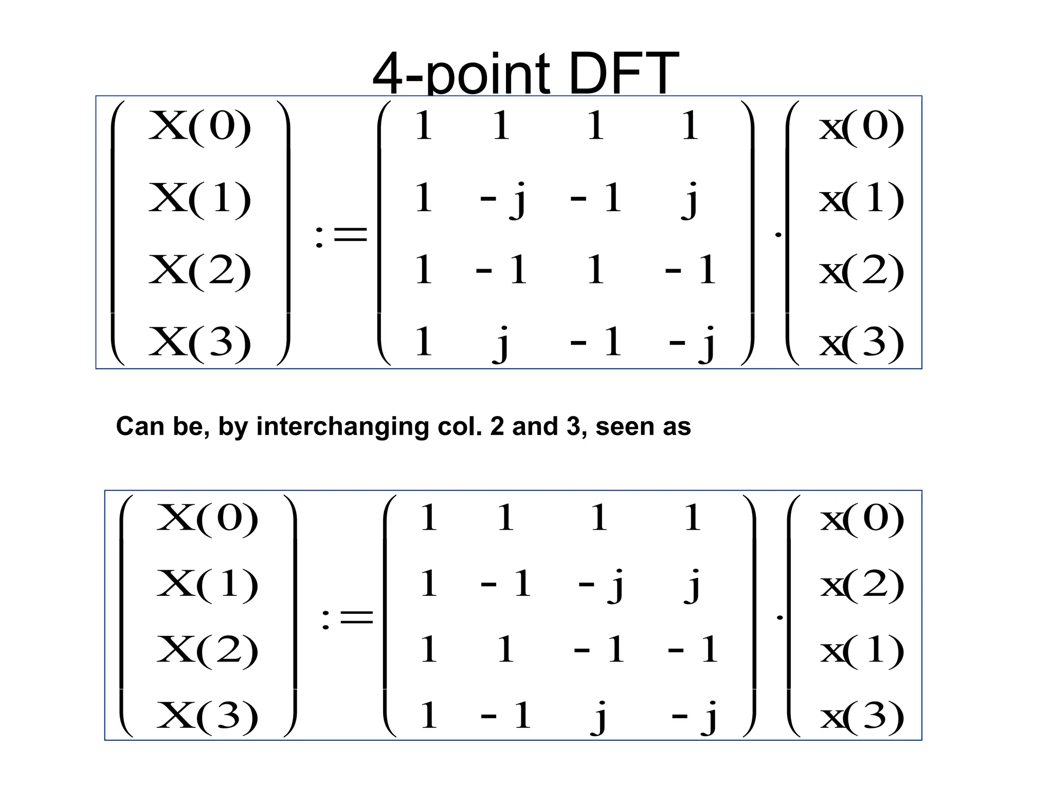
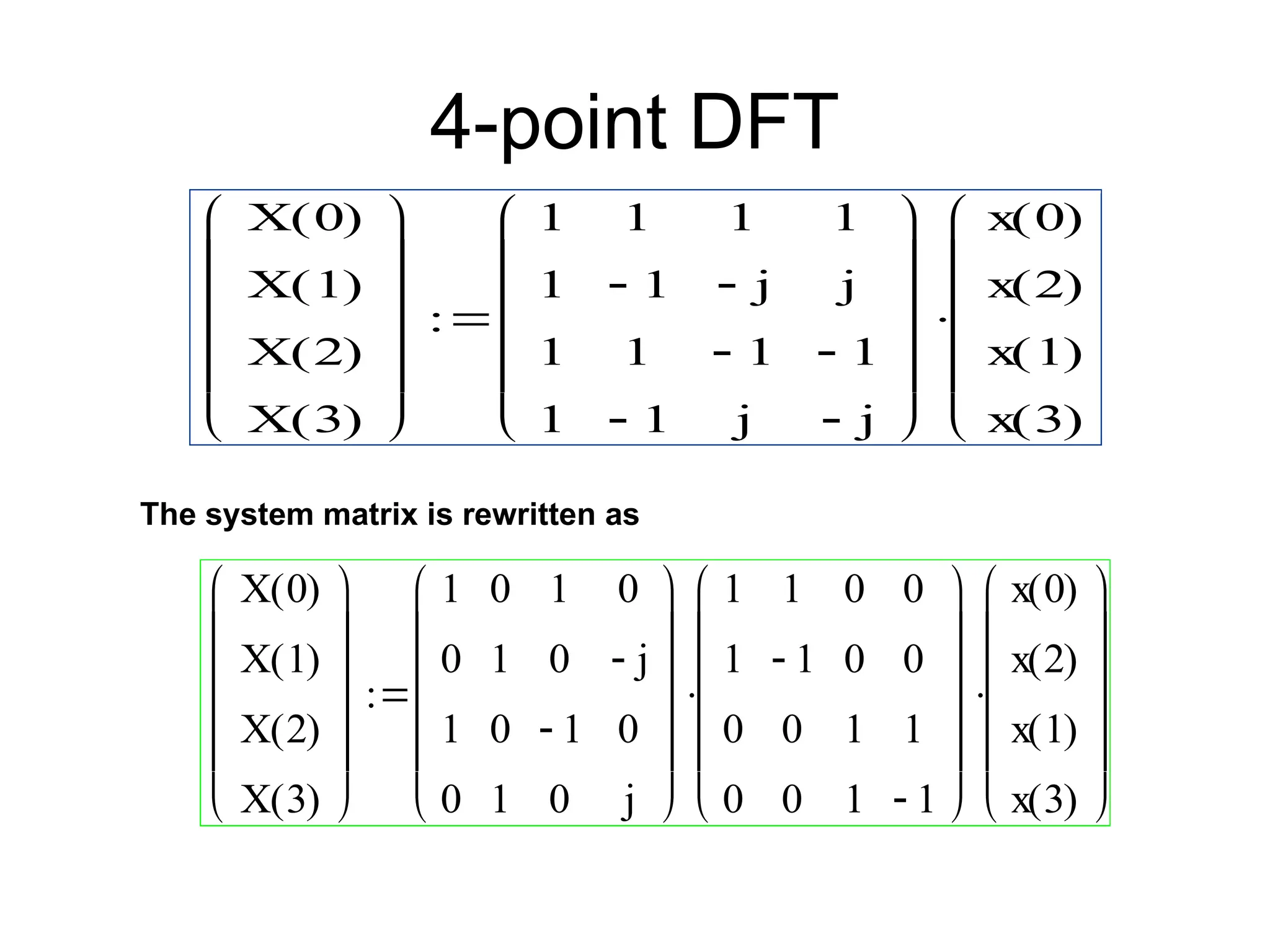
24. 4-point DFT
X 0
( )
X 1
( )
X 2
( )
X 3
( )












1
1
1
1
1
j

1

j
1
1

1
1

1
j
1

j













x 0
( )
x 1
( )
x 2
( )
x 3
( )














Can be, by interchanging col. 2 and 3, seen as
X 0
( )
X 1
( )
X 2
( )
X 3
( )












1
1
1
1
1
1

1
1

1
j

1

j
1
j
1

j













x 0
( )
x 2
( )
x 1
( )
x 3
( )















25. 4-point DFT
X 0
( )
X 1
( )
X 2
( )
X 3
( )












1
1
1
1
1
1

1
1

1
j

1

j
1
j
1

j













x 0
( )
x 2
( )
x 1
( )
x 3
( )














The system matrix is rewritten as
X 0
( )
X 1
( )
X 2
( )
X 3
( )












1
0
1
0
0
1
0
1
1
0
1

0
0
j

0
j












1
1
0
0
1
1

0
0
0
0
1
1
0
0
1
1














x 0
( )
x 2
( )
x 1
( )
x 3
( )















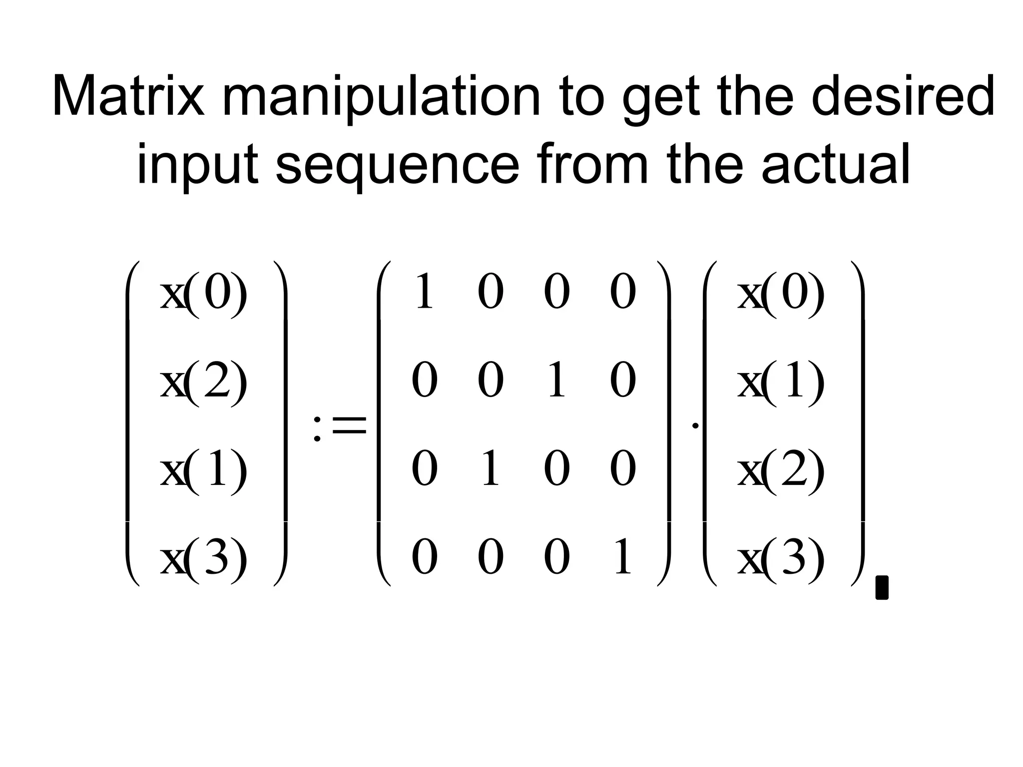
26. Matrix manipulation to get the desired
input sequence from the actual
x 0
( )
x 2
( )
x 1
( )
x 3
( )












1
0
0
0
0
0
1
0
0
1
0
0
0
0
0
1












x 0
( )
x 1
( )
x 2
( )
x 3
( )















27. Process of decimation: example
X[n]
-1
-2 1
2 3 4
5
6
7 n
X[1]
X[3]
X[5]
X[7]
X[n]
-1
-2 1
2 3 4
5
6
7 n
X[1]
X[2]
X[3] X[4]
X[5]
X[6]
X[7]
X[0]
X[n]
-1
-2 1
2 3 4
5
6
7 n
X[2]
X[4]
X[6]
X[0]
Separating the above sequence for +ve ‘n’ in even and odd sequence numbers .

28. Process of decimation: example
X[n]
-
- 1
2 3 4
5
6
7 n
X[1]
X[3]
X[5]
X[7]
2 3 4 6
X[n]
- 1 5 7 n
X[2]
X[4]
X[6]
X[0]
Compress the even sequence by two.
Shift the sequence to left by one and
compress by two
X[n]
-
1 2 3
n
X[2]
X[4]
X[6]
X[0]
X[n]
2
4 6 n
X[1]
X[3]
X[5]
X[7]
The compression is also called decimation

29. x 0
( ) x 2
( )

x 0
( ) x 2
( )

x 1
( ) x 3
( )

x 1
( ) x 3
( )













1
1
0
0
1
1

0
0
0
0
1
1
0
0
1
1













x 0
( )
x 2
( )
x 1
( )
x 3
( )














X 0
( )
X 1
( )
X 2
( )
X 3
( )












1
0
1
0
0
1
0
1
1
0
1

0
0
j

0
j












x 0
( ) x 2
( )

x 0
( ) x 2
( )

x 1
( ) x 3
( )

x 1
( ) x 3
( )















X 0
( )
X 1
( )
X 2
( )
X 3
( )












1
0
1
0
0
1
0
1
1
0
1

0
0
j

0
j












1
1
0
0
1
1

0
0
0
0
1
1
0
0
1
1














x 0
( )
x 2
( )
x 1
( )
x 3
( )













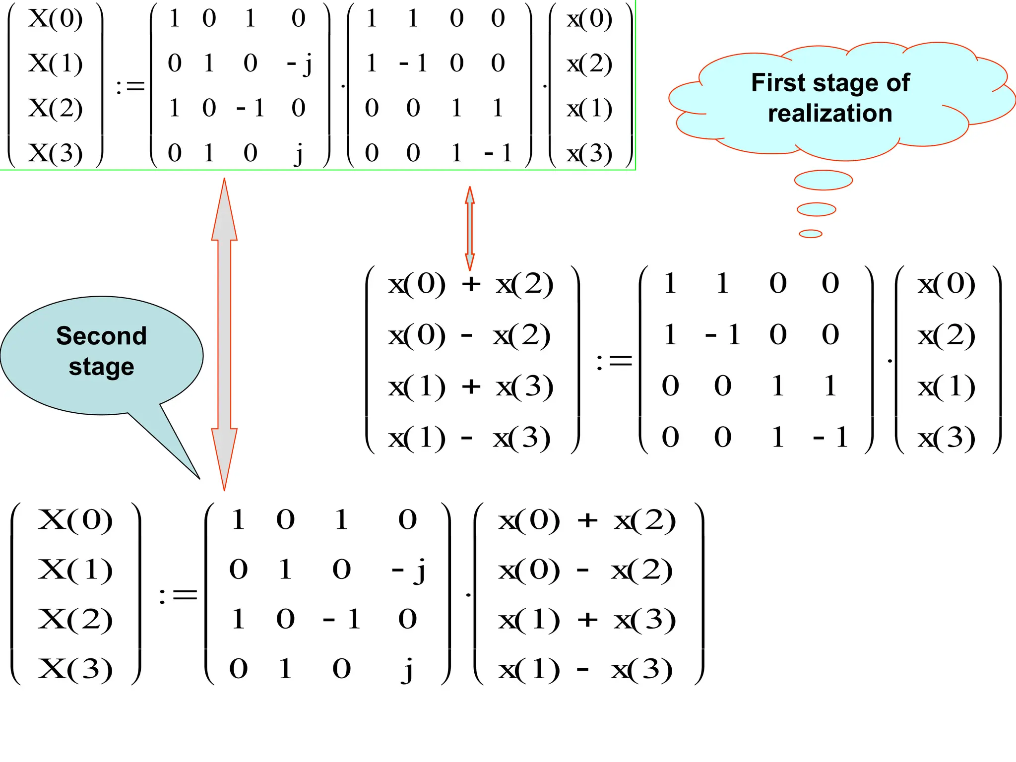
 First stage of
realization
Second
stage

30. Decimation of 4 point DFT into 2xradix-2
• The values of
W4
0
= 1; W4
2
= -1; W4
1
= -j; and W4
3
= j
X[0]
x0
x2
x1
x3
x0+x2
xo -x2
x1+x3
x1-x3
X[1]
X[2]
X[3]
Wo

w1

W2

W3

-1
-1

31. Decimation of 4 point DFT into 2xradix-2
• The values of
W4
0
= 1; W4
2
= -1; W4
1
= -j; and W4
3
= j
X[0]
N/4 point
DFT
even
N/4 point
DFT
odd
x0
x2
x1
x3
x0+x2
xo -x2
x1+x3
x1-x3
X[1]
X[2]
X[3]
Wo

w1

W2

W3


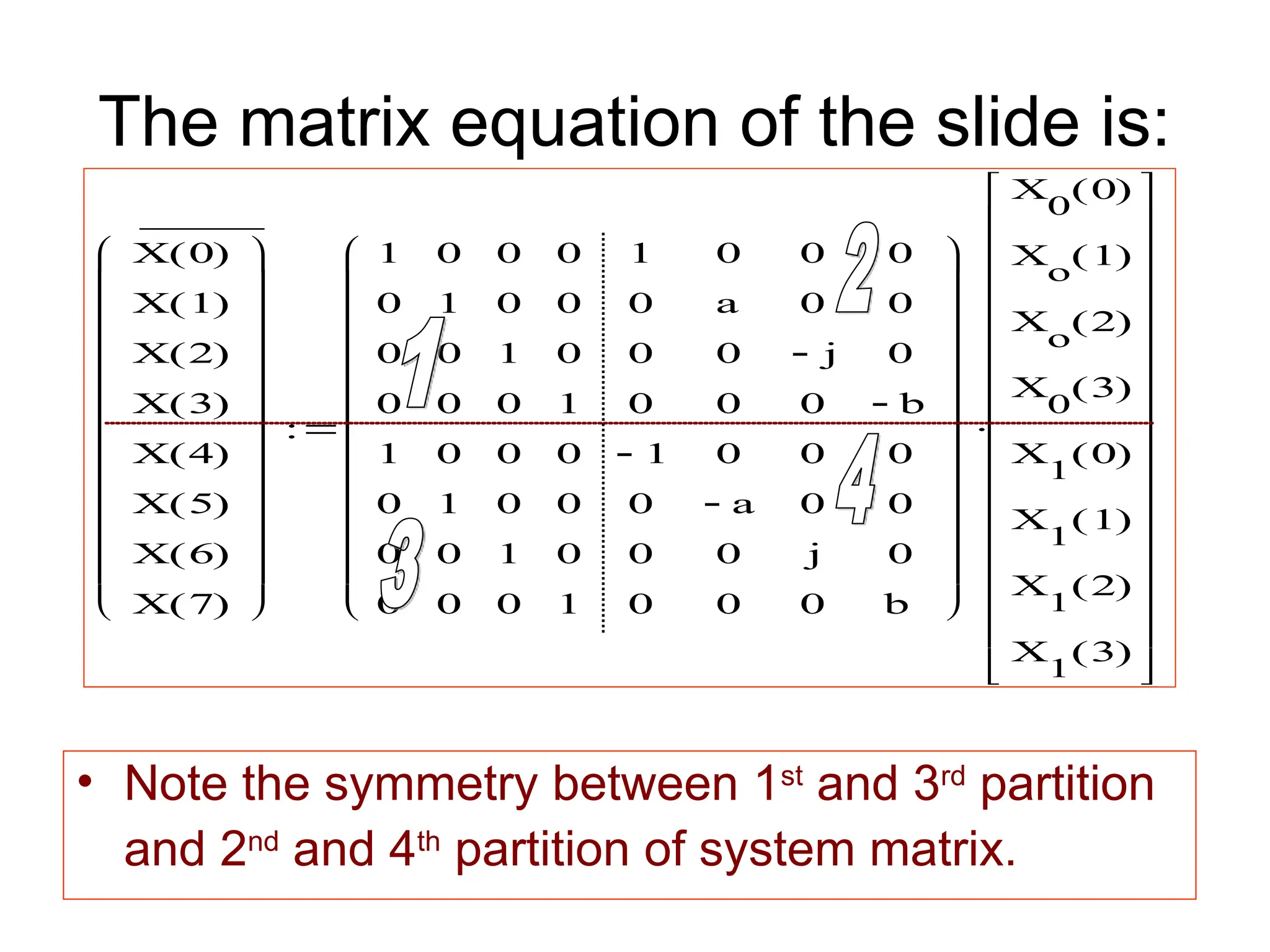
32. N=8-point radix-4 DIT-FFT:
N/2 point
DFT
[EVEN]
N/2 point
DFT
[ODD]
X(0)
X(4)
X(2)
X(6)
X(1)
X(3)
X(5)
X(7)
X[0]
X[1]
X[2]
X[3]
X[4]
X[5]
X[6]
X[7]
X0[0]
X1 [0]
X0[1]
X1 [1]
X0[2]
X1[2]
X0[3]
X1[3]
a
-j 
-b
-1
-a 
j
b
Note: -W4
= W0
=1; -W5
= W1
= a = (1-j)/2;
-W2
= W6
=j and -W3
= W7
= b = (1+j)/2
1

33. The matrix equation of the slide is:
• Note the symmetry between 1st
and 3rd
partition
and 2nd
and 4th
partition of system matrix.
X 0
( )
X 1
( )
X 2
( )
X 3
( )
X 4
( )
X 5
( )
X 6
( )
X 7
( )























1
0
0
0
1
0
0
0
0
1
0
0
0
1
0
0
0
0
1
0
0
0
1
0
0
0
0
1
0
0
0
1
1
0
0
0
1

0
0
0
0
a
0
0
0
a

0
0
0
0
j

0
0
0
j
0
0
0
0
b

0
0
0
b






















X
0
0
( )
X
o
1
( )
X
o
2
( )
X
0
3
( )
X
1
0
( )
X
1
1
( )
X
1
2
( )
X
1
3
( )

































34. N=8-point radix-2 DIT-FFT:
N-point DFT
N/2 point DFT
N/4 point DFT
X[0]
X[1]
X[2]
X[3]
X[4]
X[5]
X[6]
X[7]
x[0]
x[4]
x[2]
x[6]
x[1]
x[5]
x[3]
x[7]
-1
-1
-1
-1
-1
-1
-1
-1
w2
w2
w2
w1
w3
-1
-1
-1
-1

35. System Matrix for N/2 point DFT
Block
Note that partitions 2 and 3 are null matrices while partitions 1 and 4 are identical.
Also note that subpartitions 1st
and 3rd
are I matrices and
2nd
and 4th
sub-partitions have sign difference.
Cross diagonals in either case are zero.
X
0
0
( )
X
o
1
( )
X
o
2
( )
X
0
3
( )
X
1
0
( )
X
1
1
( )
X
1
2
( )
X
1
3
( )






























1
0
1
0
0
0
0
0
0
1
0
1
0
0
0
0
1
0
1

0
0
0
0
0
0
j

0
j
0
0
0
0
0
0
0
0
1
0
1
0
0
0
0
0
0
1
0
1
0
0
0
0
1
0
1

0
0
0
0
0
0
j

0
j






















x 0
( ) x 4
( )

x 0
( ) x 4
( )

x 2
( ) x 6
( )

x 2
( ) x 6
( )

x 1
( ) x 5
( )

x 1
( ) x 5
( )

x 3
( ) x 7
( )

x 3
( ) x 7
( )


























36. System Matrix for N/4 block
Again see the simile between 1and 4 partitions. Note that 2 and 3 s are null matrices.
Further note the sub-partition matrices. They also follow the same rule. All
the elements are real.
x 0
( ) x 4
( )

x 0
( ) x 4
( )

x 2
( ) x 6
( )

x 2
( ) x 6
( )

x 1
( ) x 5
( )

x 1
( ) x 5
( )

x 3
( ) x 7
( )

x 3
( ) x 7
( )























1
1
0
0
0
0
0
0
1
1

0
0
0
0
0
0
0
0
1
1
0
0
0
0
0
0
1
1

0
0
0
0
0
0
0
0
1
1
0
0
0
0
0
0
1
1

0
0
0
0
0
0
0
0
1
1
0
0
0
0
0
0
1
1























x 1
( )
x 4
( )
x 2
( )
x 6
( )
x 1
( )
x 5
( )
x 3
( )
x 7
( )

























37. Signal flow graph for decimation of 8 point DFT
N-point DFT
N/2 point DFT
N/4 point DFT
X[0]
X[1]
X[2]
X[3]
X[4]
X[5]
X[6]
X[7]
x[0]
x[4]
x[2]
x[6]
x[1]
x[5]
x[3]
x[7]
-1
-1
-1
-1
-1
-1
-1
-1
w2
w2
w2
w1
w3
-1
-1
-1
-1