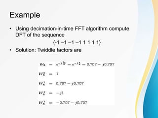
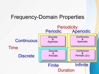
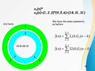
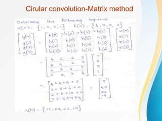
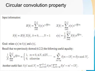
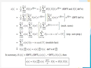
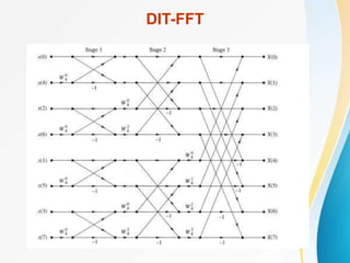
The document discusses discrete Fourier transforms (DFT). It begins with an overview of the syllabus which includes discrete signals and systems, introduction to DFT, properties of DFT, and applications of DFT such as filtering and fast Fourier transform (FFT) algorithms. It then provides background on digital signal processing, discussing how analog signals are converted to digital signals using sampling and then processed digitally before being reconstructed back to analog signals. The benefits and limitations of digital versus analog signal processing are also summarized.

![Discrete-Time Signals: Sequences
• Discrete-time signals are represented by sequence of numbers
– The nth number in the sequence is represented with x[n]
• Often times sequences are obtained by sampling of continuous-time signals
– In this case x[n] is value of the analog signal at xc(nT)
– Where T is the sampling period
0 20 40 60 80 100
-10
0
10
t (ms)
0 10 20 30 40 50
-10
0
10
n (samples)](https://image.slidesharecdn.com/unit11-231016135759-01e1b996/85/unit-11-ppt-12-320.jpg)
![Basic Sequences and Operations
• Delaying (Shifting) a sequence
• Unit sample (impulse) sequence
• Unit step sequence
• Exponential sequences
]
n
n
[
x
]
n
[
y o
0
n
1
0
n
0
]
n
[
0
n
1
0
n
0
]
n
[
u
n
A
]
n
[
x
-10 -5 0 5 10
0
0.5
1
1.5
-10 -5 0 5 10
0
0.5
1
1.5
-10 -5 0 5 10
0
0.5
1](https://image.slidesharecdn.com/unit11-231016135759-01e1b996/85/unit-11-ppt-13-320.jpg)
![Sinusoidal Sequences
• Important class of sequences
• An exponential sequence with complex
• x[n] is a sum of weighted sinusoids
• Different from continuous-time, discrete-time sinusoids
– Have ambiguity of 2k in frequency
– Are not necessary periodic with 2/o
n
cos
n
x o
j
j
e
A
A
and
e o
n
sin
A
j
n
cos
A
n
x
e
A
e
e
A
A
n
x
o
n
o
n
n
j
n
n
j
n
j
n o
o
n
cos
n
k
2
cos o
o
integer
an
is
k
2
N
if
only
N
n
cos
n
cos
o
o
o
o
](https://image.slidesharecdn.com/unit11-231016135759-01e1b996/85/unit-11-ppt-14-320.jpg)
![Discrete-Time Systems
• Discrete-Time Sequence is a mathematical operation that maps a given
input sequence x[n] into an output sequence y[n]
• Example Discrete-Time Systems
– Moving (Running) Average
– Maximum
– Ideal Delay System
]}
n
[
x
{
T
]
n
[
y T{.}
x[n] y[n]
]
3
n
[
x
]
2
n
[
x
]
1
n
[
x
]
n
[
x
]
n
[
y
]
2
n
[
x
],
1
n
[
x
],
n
[
x
max
]
n
[
y
]
n
n
[
x
]
n
[
y o
](https://image.slidesharecdn.com/unit11-231016135759-01e1b996/85/unit-11-ppt-16-320.jpg)
![Memoryless System
• Memoryless System
– A system is memoryless if the output y[n] at every value of n
depends only on the input x[n] at the same value of n
• Example Memoryless Systems
– Square
– Sign
• Counter Example
– Ideal Delay System
2
]
n
[
x
]
n
[
y
]
n
[
x
sign
]
n
[
y
]
n
n
[
x
]
n
[
y o
](https://image.slidesharecdn.com/unit11-231016135759-01e1b996/85/unit-11-ppt-17-320.jpg)
![Linear Systems
• Linear System: A system is linear if and only if
• Examples
– Ideal Delay System
(scaling)
]
n
[
x
aT
]
n
[
ax
T
and
y)
(additivit
]
n
[
x
T
]
n
[
x
T
]}
n
[
x
]
n
[
x
{
T 2
1
2
1
]
n
n
[
x
]
n
[
y o
]
n
n
[
ax
]
n
[
x
aT
]
n
n
[
ax
]
n
[
ax
T
]
n
n
[
x
]
n
n
[
x
]
n
[
x
T
]}
n
[
x
{
T
]
n
n
[
x
]
n
n
[
x
]}
n
[
x
]
n
[
x
{
T
o
1
o
1
o
2
o
1
1
2
o
2
o
1
2
1
](https://image.slidesharecdn.com/unit11-231016135759-01e1b996/85/unit-11-ppt-18-320.jpg)
![Time-Invariant Systems
• Time-Invariant (shift-invariant) Systems
– A time shift at the input causes corresponding time-shift at output
• Example
– Square
• Counter Example
– Compressor System
]
n
n
[
x
T
]
n
n
[
y
]}
n
[
x
{
T
]
n
[
y o
o
2
]
n
[
x
]
n
[
y
2
o
o
2
o
1
]
n
n
[
x
n
-
n
y
gives
output
the
Delay
]
n
n
[
x
n
y
is
output
the
input
the
Delay
]
Mn
[
x
]
n
[
y
o
o
o
1
n
n
M
x
n
-
n
y
gives
output
the
Delay
]
n
Mn
[
x
n
y
is
output
the
input
the
Delay
](https://image.slidesharecdn.com/unit11-231016135759-01e1b996/85/unit-11-ppt-19-320.jpg)
![Causal System
• Causality
– A system is causal it’s output is a function of
only the current and previous samples
• Examples
– Backward Difference
• Counter Example
– Forward Difference
]
n
[
x
]
1
n
[
x
]
n
[
y
]
1
n
[
x
]
n
[
x
]
n
[
y
](https://image.slidesharecdn.com/unit11-231016135759-01e1b996/85/unit-11-ppt-20-320.jpg)
![Stable System
• Stability (in the sense of bounded-input bounded-output BIBO)
– A system is stable if and only if every bounded input produces a
bounded output
• Example
– Square
• Counter Example
– Log
y
x B
]
n
[
y
B
]
n
[
x
2
]
n
[
x
]
n
[
y
2
x
x
B
]
n
[
y
by
bounded
is
output
B
]
n
[
x
by
bounded
is
input
if
]
n
[
x
log
]
n
[
y 10
n
x
log
0
y
0
n
x
for
bounded
not
output
B
]
n
[
x
by
bounded
is
input
if
even
10
x](https://image.slidesharecdn.com/unit11-231016135759-01e1b996/85/unit-11-ppt-21-320.jpg)
![Linear Time Invariant (LTI) Systems and z-Transform
]
[n
x ]
[n
y
]
[n
h
If the system is LTI we compute the output with the convolution:
m
m
n
x
m
h
n
x
n
h
n
y ]
[
]
[
]
[
*
]
[
]
[
If the impulse response has a finite duration, the system is called FIR (Finite Impulse
Response):
]
[
]
[
...
]
1
[
]
1
[
]
[
]
0
[
]
[ N
n
x
N
h
n
x
h
n
x
h
n
y
](https://image.slidesharecdn.com/unit11-231016135759-01e1b996/85/unit-11-ppt-24-320.jpg)
![
n
n
z
n
x
n
x
Z
z
X ]
[
]
[
)
(
Z-Transform
Facts:
)
(
)
(
)
( z
X
z
H
z
Y
]
[n
x ]
[n
y
)
(z
H
Frequency Response of a filter:
f
j
e
z
z
H
f
H
2
)
(
)
(
](https://image.slidesharecdn.com/unit11-231016135759-01e1b996/85/unit-11-ppt-25-320.jpg)
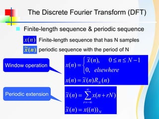
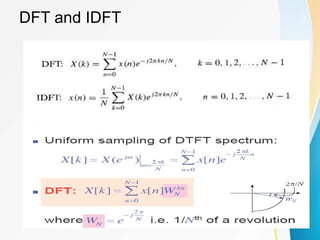
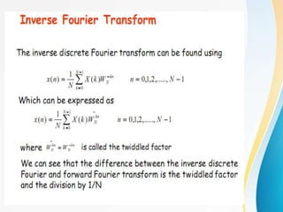
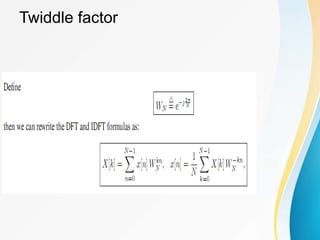
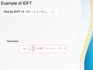
![ The definition of DFT
The Discrete Fourier Transform (DFT)
1
0
,
)
(
1
)]
(
[
IDFT
)
(
1
0
,
)
(
)]
(
[
DFT
)
(
1
0
1
0
N
n
W
k
X
N
k
X
n
x
N
k
W
n
x
n
x
k
X
N
n
nk
N
N
n
nk
N
)
(
)
(
~
)
(
)
(
1
)
(
)
(
)
(
~
)
(
)
(
)
(
1
0
1
0
n
R
n
x
n
R
W
k
X
N
n
x
k
R
k
X
k
R
W
n
x
k
X
N
N
n
N
nk
N
N
N
n
N
nk
N
](https://image.slidesharecdn.com/unit11-231016135759-01e1b996/85/unit-11-ppt-38-320.jpg)
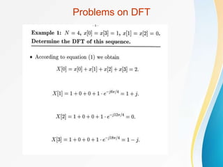
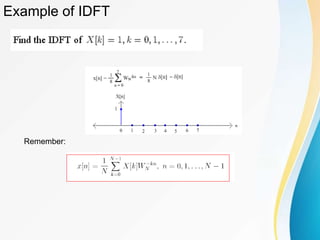
![Example of DFT
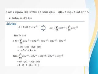
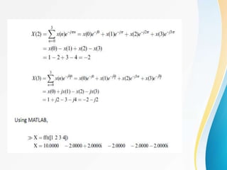
• Find X[k]
– We know k=1,.., 7; N=8](https://image.slidesharecdn.com/unit11-231016135759-01e1b996/85/unit-11-ppt-44-320.jpg)

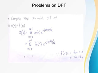
![Example of DFT
Summation for X[k]
Using the shift property!](https://image.slidesharecdn.com/unit11-231016135759-01e1b996/85/unit-11-ppt-49-320.jpg)
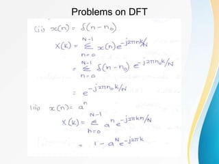
![Example of DFT
Summation for X[k]
Using the shift property!](https://image.slidesharecdn.com/unit11-231016135759-01e1b996/85/unit-11-ppt-50-320.jpg)
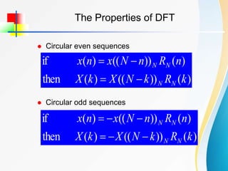
![The Properties of DFT
Linearity
)
(
)
(
)]
(
)
(
[
DFT 2
1
2
1 k
bX
k
aX
n
bx
n
ax
N3-point DFT, N3=max(N1,N2)
Circular shift of a sequence
)
(
)]
(
))
((
[
DFT k
X
W
n
R
m
n
x km
N
N
N
)
(
))
((
)]
(
[
DFT k
R
l
k
X
n
x
W N
N
nl
N
Circular shift in the frequency domain](https://image.slidesharecdn.com/unit11-231016135759-01e1b996/85/unit-11-ppt-62-320.jpg)
![The Properties of DFT
The sum of a sequence
1
0
0
1
0
0
)
(
)
(
)
(
N
n
k
N
n
nk
N
k
n
x
W
n
x
k
X
The first sample of sequence
1
0
)
(
1
)
0
(
N
k
k
X
N
x
)
(
))
((
)]
(
[
)
(
)]
(
[
k
R
k
N
Nx
n
X
DFT
k
X
n
x
DFT
N
N
](https://image.slidesharecdn.com/unit11-231016135759-01e1b996/85/unit-11-ppt-63-320.jpg)
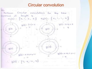
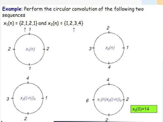
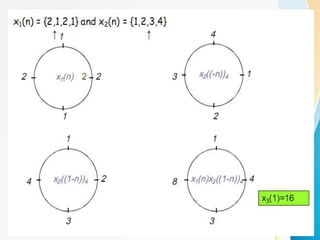
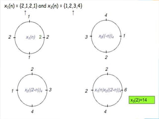
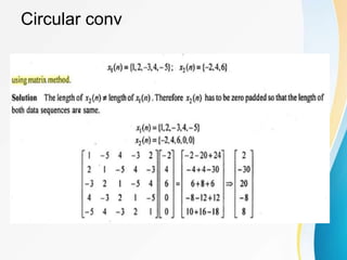
![The Properties of DFT
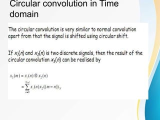
Circular convolution
)
(
)
(
)
(
))
((
)
(
)
(
))
((
)
(
)
(
)
(
1
2
1
0
1
2
1
0
2
1
2
1
n
x
n
x
n
R
m
n
x
m
x
n
R
m
n
x
m
x
n
x
n
x
N
N
m
N
N
N
m
N
N
N
)
(
)
(
)]
(
)
(
[
DFT 2
1
2
1 k
X
k
X
n
x
n
x
N
)
(
)
(
1
)]
(
)
(
[
DFT 2
1
2
1 k
X
k
X
N
n
x
n
x
N
Multiplication](https://image.slidesharecdn.com/unit11-231016135759-01e1b996/85/unit-11-ppt-64-320.jpg)
![The Properties of DFT
Circular convolution
)
(
)
(
)
(
))
((
)
(
)
(
))
((
)
(
)
(
)
(
1
2
1
0
1
2
1
0
2
1
2
1
n
x
n
x
n
R
m
n
x
m
x
n
R
m
n
x
m
x
n
x
n
x
N
N
m
N
N
N
m
N
N
N
)
(
)
(
)]
(
)
(
[
DFT 2
1
2
1 k
X
k
X
n
x
n
x
N
)
(
)
(
1
)]
(
)
(
[
DFT 2
1
2
1 k
X
k
X
N
n
x
n
x
N
Multiplication](https://image.slidesharecdn.com/unit11-231016135759-01e1b996/85/unit-11-ppt-65-320.jpg)
![The Properties of DFT
)
(
)
(
*
))
((
)
(
))
((
*
)
(
)]
(
[
IDFT
)
(
)
(
)
(
)
(
1
0
1
0
*
m
R
n
y
m
n
x
m
R
m
n
y
n
x
k
R
m
r
then
k
Y
k
X
k
R
if
N
N
n
N
N
N
n
N
xy
xy
xy
](https://image.slidesharecdn.com/unit11-231016135759-01e1b996/85/unit-11-ppt-67-320.jpg)
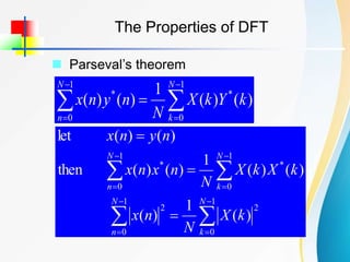
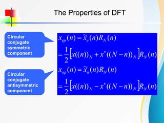
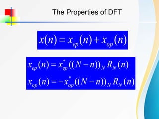
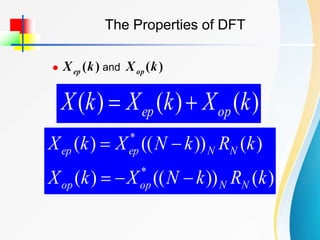
![The Properties of DFT
Conjugate symmetry properties of DFT
and
)
(n
xep )
(n
xop
Let be a N-point sequence
)
(n
x N
n
x
n
x ))
((
)
(
~
]
))
((
))
((
[
2
1
)]
(
~
)
(
~
[
2
1
)
(
~
]
))
((
))
((
[
2
1
)]
(
~
)
(
~
[
2
1
)
(
~
N
N
o
N
N
e
n
N
x
n
x
n
x
n
x
n
x
n
N
x
n
x
n
x
n
x
n
x
It can be proved that
)
(
~
)
(
~
)
(
~
)
(
~
*
*
n
x
n
x
n
x
n
x
o
o
e
e
](https://image.slidesharecdn.com/unit11-231016135759-01e1b996/85/unit-11-ppt-69-320.jpg)
![The Properties of DFT
)]
(
))
((
Im[
)]
(
Im[
)]
(
))
((
Re[
)]
(
Re[
k
R
k
N
X
k
X
k
R
k
N
X
k
X
N
N
ep
ep
N
N
ep
ep
)]
(
))
((
Im[
)]
(
Im[
)]
(
))
((
Re[
)]
(
Re[
k
R
k
N
X
k
X
k
R
k
N
X
k
X
N
N
op
op
N
N
op
op
](https://image.slidesharecdn.com/unit11-231016135759-01e1b996/85/unit-11-ppt-73-320.jpg)
![Use of DFT in linear filtering
1
0
]
[
]
[
]
[
L
k
k
n
h
k
x
n
y
DFT- based filtering always performs circular convolution.
But by zero padding adequetly,Circular convoltion can
yield the same result.
where n=0.....(L+M-1)-1](https://image.slidesharecdn.com/unit11-231016135759-01e1b996/85/unit-11-ppt-93-320.jpg)
![Linear convolution using DFT
1
]
[
]
[
)
( 2
1
L
L
N
of
length
to
n
h
and
n
x
padding
zero
a](https://image.slidesharecdn.com/unit11-231016135759-01e1b996/85/unit-11-ppt-94-320.jpg)
![]
[
*
]
[
]
[
)
( n
h
n
x
n
y
a
(2) calculate linear convolution by circular convolution
1
]
[
]
[
)
( 2
1
L
L
N
of
length
to
n
h
and
n
x
padding
zero
a
1
]
[
]
[
)
( 2
1
L
L
N
of
length
to
n
h
and
n
x
padding
zero
a
(1)calculate N point circular convolution by linear convolution
(3) calculate linear convolution by DFT
]
[
]
[
]
[
)
](
[
)
( n
R
rN
n
y
n
h
N
n
x
b N
r
]
[
)
](
[
]
[
]
[
)
( n
h
N
n
x
n
h
n
x
b
]
[
]
[
int
)
( n
h
and
n
x
of
D FT
s
po
N
b
]
[
)
](
[
]
[
*
]
[
]}
[
]
[
{
]
[
)
](
[
)
(
n
h
N
n
x
n
h
n
x
k
H
k
X
IDFT
n
h
N
n
x
c
LINEAR & CIRCULAR CONVOLUTION](https://image.slidesharecdn.com/unit11-231016135759-01e1b996/85/unit-11-ppt-95-320.jpg)

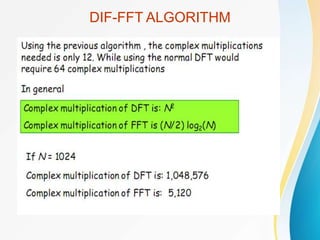
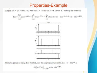
![Discrete Fourier Transform
• The DFT pair was given as
• Baseline for computational complexity:
– Each DFT coefficient requires
• N complex multiplications
• N-1 complex additions
– All N DFT coefficients require
• N2 complex multiplications
• N(N-1) complex additions
• Complexity in terms of real operations
• 4N2 real multiplications
• 2N(N-1) real additions
• Most fast methods are based on symmetry properties
– Conjugate symmetry
– Periodicity in n and k
1
N
0
k
kn
N
/
2
j
e
k
X
N
1
]
n
[
x
1
N
0
n
kn
N
/
2
j
e
]
n
[
x
k
X
kn
N
j
n
k
N
j
kN
N
j
n
N
k
N
j
e
e
e
e /
2
/
2
/
2
/
2
n
N
k
N
j
N
n
k
N
j
kn
N
j
e
e
e
/
2
/
2
/
2
](https://image.slidesharecdn.com/unit11-231016135759-01e1b996/85/unit-11-ppt-99-320.jpg)
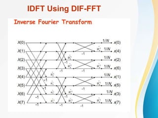
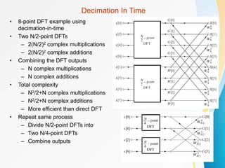
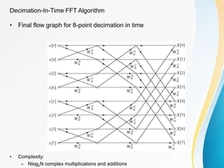
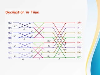
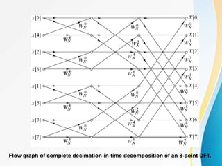
![Decimation-In-Time FFT Algorithms
• Makes use of both symmetry and periodicity
• Consider special case of N an integer power of 2
• Separate x[n] into two sequence of length N/2
– Even indexed samples in the first sequence
– Odd indexed samples in the other sequence
• Substitute variables n=2r for n even and n=2r+1 for odd
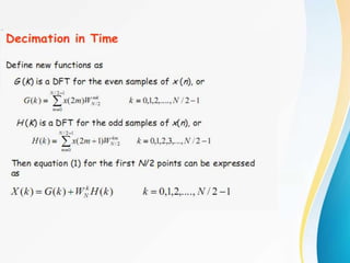
• G[k] and H[k] are the N/2-point DFT’s of each subsequence
1
odd
n
/
2
1
even
n
/
2
1
0
/
2
]
[
]
[
]
[
N
kn
N
j
N
kn
N
j
N
n
kn
N
j
e
n
x
e
n
x
e
n
x
k
X
k
H
W
k
G
W
r
x
W
W
r
x
W
r
x
W
r
x
k
X
k
N
N
rk
N
k
N
N
rk
N
N
k
r
N
N
rk
N
]
1
2
[
]
2
[
]
1
2
[
]
2
[
1
2
/
0
r
2
/
1
2
/
0
r
2
/
1
2
/
0
r
1
2
1
2
/
0
r
2](https://image.slidesharecdn.com/unit11-231016135759-01e1b996/85/unit-11-ppt-101-320.jpg)
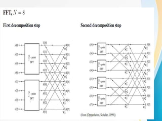
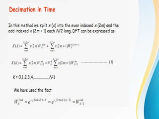
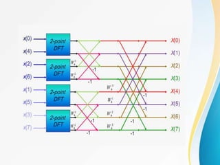
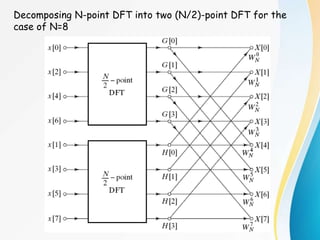
![Decimation-in-time FFT algorithm
Most conveniently illustrated by considering the special case of N
an integer power of 2, i.e, N=2v.
Since N is an even integer, we can consider computing X[k] by
separating x[n] into two (N/2)-point sequence consisting of the
even numbered point in x[n] and the odd-numbered points in x[n].
or, with the substitution of variable n=2r for n even and n=2r+1
for n odd
dd
]
[
]
[
]
[
o
n
nk
N
even
n
nk
N W
n
x
W
n
x
k
X
1
)
2
/
(
0
)
1
2
(
1
)
2
/
(
0
2
]
1
2
[
]
2
[
]
[
N
r
k
r
N
N
r
rk
N W
r
x
W
r
x
k
X
1
)
2
/
(
0
2
1
)
2
/
(
0
2
)
](
1
2
[
)
](
2
[
N
r
rk
N
k
N
N
r
rk
N W
r
x
W
W
r
x](https://image.slidesharecdn.com/unit11-231016135759-01e1b996/85/unit-11-ppt-113-320.jpg)
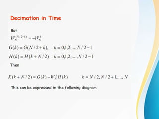
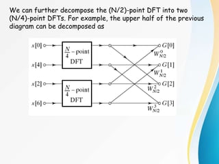
![Since
That is, WN
2 is the root of the equation WN/2=1
Consequently,
Both G[k] and H[k] can be computed by (N/2)-point DFT, where
G[k] is the (N/2)-point DFT of the even numbered points of the
original sequence and the second being the (N/2)-point DFT of
the odd-numbered point of the original sequence.
Although the index ranges over N values, k = 0, 1, …, N-1, each of
the sums must be computed only for k between 0 and (N/2)-1,
since G[k] and H[k] are each periodic in k with period N/2.
2
/
)
2
/
/(
2
)
/
2
(
2
2
N
N
j
N
j
N W
e
e
W
1
,...,
1
,
0
],
[
]
[
N
k
k
H
W
k
G k
N
1
)
2
/
(
0
2
1
)
2
/
(
0
2
)
](
1
2
[
)
](
2
[
]
[
N
r
rk
N
k
N
N
r
rk
N W
r
x
W
W
r
x
k
X](https://image.slidesharecdn.com/unit11-231016135759-01e1b996/85/unit-11-ppt-114-320.jpg)
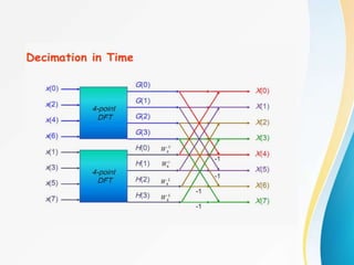
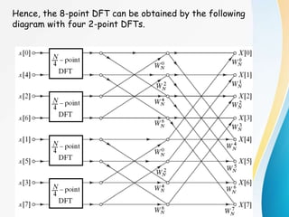
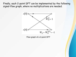
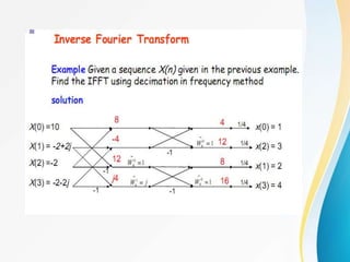
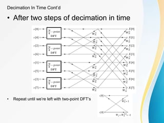
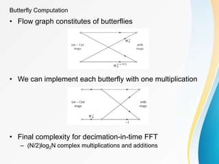
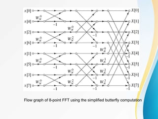
![In each stage of the decimation-in-time FFT algorithm, there
are a basic structure called the butterfly computation:
The butterfly computation can be simplified as follows:
Flow graph of a basic butterfly
computation in FFT.
Simplified butterfly computation.
]
[
]
[
]
[
]
[
]
[
]
[
1
1
1
1
q
X
W
p
X
q
X
q
X
W
p
X
p
X
m
r
N
m
m
m
r
N
m
m
](https://image.slidesharecdn.com/unit11-231016135759-01e1b996/85/unit-11-ppt-124-320.jpg)
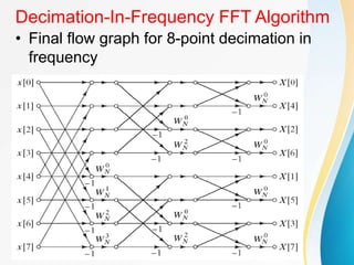
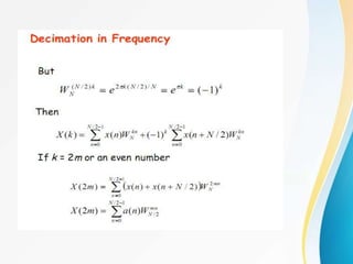
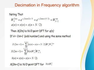
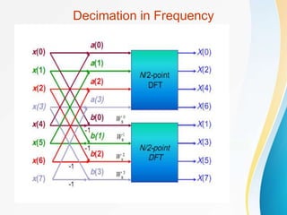
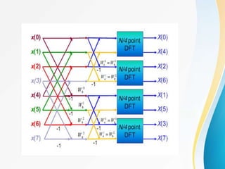
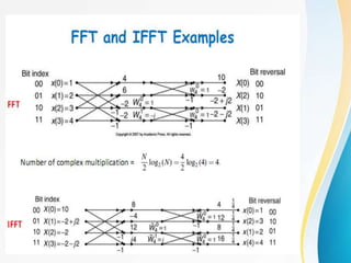
![Decimation-In-Frequency FFT Algorithm
• The DFT equation
• Split the DFT equation into even and odd
frequency indexes
• Substitute variables to get
• Similarly for odd-numbered frequencies
1
N
0
n
nk
N
W
]
n
[
x
k
X
1
2
/
2
1
2
/
0
2
1
0
2
]
[
]
[
]
[
2
N
N
n
r
n
N
N
n
r
n
N
N
n
r
n
N W
n
x
W
n
x
W
n
x
r
X
1
2
/
0
2
/
1
2
/
0
2
2
/
1
2
/
0
2
]
2
/
[
]
[
]
2
/
[
]
[
2
N
n
nr
N
N
n
r
N
n
N
N
n
r
n
N W
N
n
x
n
x
W
N
n
x
W
n
x
r
X
1
2
/
0
1
2
2
/
]
2
/
[
]
[
1
2
N
n
r
n
N
W
N
n
x
n
x
r
X](https://image.slidesharecdn.com/unit11-231016135759-01e1b996/85/unit-11-ppt-129-320.jpg)